
Concept explainers
Videos
A very large batch of components has arrived at a distributor. The batch can be characterized as accept-able only if the proportion of defective components is at most .10. The distributor decides to randomly select 10 components and to accept the batch only if the number of defective components in the sample is at most 2.
- a. What is the
probability that the batch will be accepted when the actual proportion of defectives is .01? .05? .10? .20? .25? - b. Let p denote the actual proportion of defectives in the batch. A graph of P(batch is accepted) as a
function of p, with p on the horizontal axis and P(batch is accepted) on the vertical axis, is called the operating characteristic curve for the acceptance sampling plan. Use the results of part (a) to sketch this curve for 0 ≤ p ≤ 1. - c. Repeat parts (a) and (b) with “1” replacing “2” in the acceptance sampling plan.
- d. Repeat parts (a) and (b) with “15” replacing “10” in the acceptance sampling plan.
- e. Which of the three sampling plans, that of part (a), (c), or (d), appears most satisfactory, and why?
a.
Find the probability that the batch will be accepted when the actual proportion of defectives is 0.01, 0.05, 0.10, 0.20 and 0.25.
Answer to Problem 58E
The probability that the batch will be accepted for different values of actual proportion of defectives, are,
| p | |
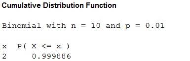
| 0.01 | 0.998 |
| 0.05 | 0.9885 |
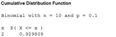
| 0.1 | 0.9298 |
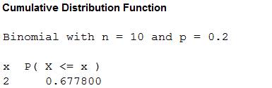
| 0.20 | 0.6778 |
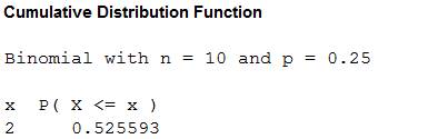
| 0.25 | 0.5256 |
Explanation of Solution
Given info:
A distributor decided to select 10 components randomly from a batch. The batch will be accepted if the number of defective components in the sample is at most 2. A batch is characterized as acceptable if the proportion of defective components is at most 0.10.
Calculation:
Let p be the actual proportion of defective in the batch.
Let X be the number of defectives in the sample.
The sample size is 10. The samples are selected randomly and the outcomes are defective or non-defective.
Hence,
It is given that the batch will be accepted if the number of defective components in the sample is at most 2 means the batch will be accepted if
The probability that the batch will be accepted when the actual proportion of defectives is p, is
The probability values:
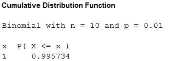
For p = 0.01:
Software procedure:
Step by step procedure to obtain the probability values using the MINITAB software:
- Choose Calc > Probability Distribution> Binomial Distribution.
- Enter number of trials as 10 and event probability as 0.01.
- Choose Cumulative probability.
- In Input constant, enter 2.
- Click OK.
Output using MINITAB software is given below:
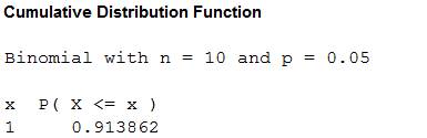
For p = 0.05:
Software procedure:
Step by step procedure to obtain the probability values using the MINITAB software:
- Choose Calc > Probability Distribution> Binomial Distribution.
- Enter number of trials as 10 and event probability as 0.05
- Choose Cumulative probability.
- In Input constant, enter 2.
- Click OK.
Output using MINITAB software is given below:

For p = 0.10:
Software procedure:
Step by step procedure to obtain the probability values using the MINITAB software:
- Choose Calc > Probability Distribution> Binomial Distribution.
- Enter number of trials as 10 and event probability as 0.10
- Choose Cumulative probability.
- In Input constant, enter 2.
- Click OK.
Output using MINITAB software is given below:
For p = 0.2:
Software procedure:
Step by step procedure to obtain the probability values using the MINITAB software:
- Choose Calc > Probability Distribution> Binomial Distribution.
- Enter number of trials as 10 and event probability as 0.20
- Choose Cumulative probability.
- In Input constant, enter 2.
- Click OK.
Output using MINITAB software is given below:
For p = 0.25:
Software procedure:
Step by step procedure to obtain the probability values using the MINITAB software:
- Choose Calc > Probability Distribution> Binomial Distribution.
- Enter number of trials as 10 and event probability as 0.25
- Choose Cumulative probability.
- In Input constant, enter 2.
- Click OK.
Output using MINITAB software is given below:
Hence, the probability that the batch will be accepted for different values of actual proportion of defectives and for
| p | |
| 0.01 | 0.998 |
| 0.05 | 0.9885 |
| 0.1 | 0.9298 |
| 0.20 | 0.6778 |
| 0.25 | 0.5256 |
b.
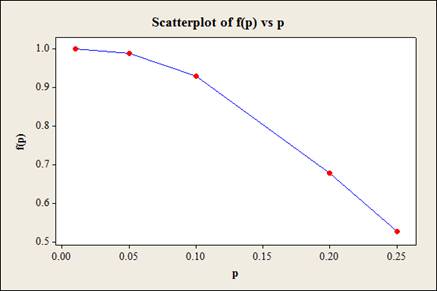
Sketch the OC curve for the accepting sampling plan.
Answer to Problem 58E
The graph is given below:
Explanation of Solution
Calculation:
From part (a) it is found that, the probability that the batch will be accepted for different values of actual proportion of defectives, are,
| p | |
| 0.01 | 0.998 |
| 0.05 | 0.9885 |
| 0.1 | 0.9298 |
| 0.20 | 0.6778 |
| 0.25 | 0.5256 |
Software procedure:
Step by step procedure to obtain the probability values using the MINITAB software:
- Choose Graph > Scatterplot.
- Choose With Connect Line, and then click OK.
- Under Y variables, enter a column of f(p).
- Under X variables, enter a column of p.
- Click OK.
Output using MINITAB software is given below:
c.
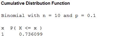
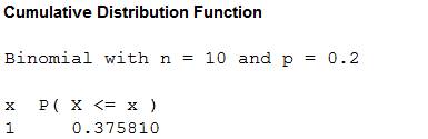
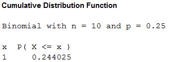
Find the probability that the batch will be accepted when the actual proportion of defectives is 0.01, 0.05, 0.10, 0.20 and 0.25 with “1” replacing “2”.
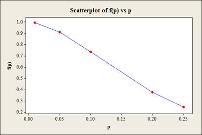
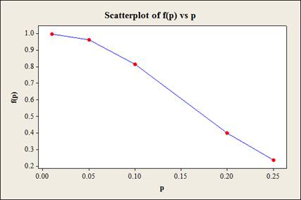
Sketch the OC curve for the accepting sampling plan.
Answer to Problem 58E
The probability that the batch will be accepted when the actual proportion of defectives is 0.01, 0.05, 0.10, 0.20 and 0.25 are 0.9957, 0.9138, 0.7360, 0.3758, and 0.2440 respectively.
The OC curve is given below
Explanation of Solution
Given info:
The c value 2 is replaced by 1.
Calculation:
Let p be the actual proportion of defective in the batch.
Let X be the number of defectives in the sample.
The sample size is 10. The samples are selected randomly and the outcomes are defective or non-defective.
Hence,
It is given that the batch will be accepted if the number of defective components in the sample is at most 1 means the batch will be accepted if
The probability that the batch will be accepted when the actual proportion of defectives is p, is
The probability values:
For p = 0.01:
Software procedure:
Step by step procedure to obtain the probability values using the MINITAB software:
- Choose Calc > Probability Distribution> Binomial Distribution.
- Enter number of trials as 10 and event probability as 0.01
- Choose Cumulative probability.
- In Input constant, enter 1.
- Click OK.
Output using MINITAB software is given below:
For p = 0.05:
Software procedure:
Step by step procedure to obtain the probability values using the MINITAB software:
- Choose Calc > Probability Distribution> Binomial Distribution.
- Enter number of trials as 10 and event probability as 0.05
- Choose Cumulative probability.
- In Input constant, enter 1.
- Click OK.
Output using MINITAB software is given below:
For p = 0.10:
Software procedure:
Step by step procedure to obtain the probability values using the MINITAB software:
- Choose Calc > Probability Distribution> Binomial Distribution.
- Enter number of trials as 10 and event probability as 0.10
- Choose Cumulative probability.
- In Input constant, enter 1.
- Click OK.
Output using MINITAB software is given below:
For p = 0.2:
Software procedure:
Step by step procedure to obtain the probability values using the MINITAB software:
- Choose Calc > Probability Distribution> Binomial Distribution.
- Enter number of trials as 10 and event probability as 0.20
- Choose Cumulative probability.
- In Input constant, enter 1.
- Click OK.
Output using MINITAB software is given below:
For p = 0.25:
Software procedure:
Step by step procedure to obtain the probability values using the MINITAB software:
- Choose Calc > Probability Distribution> Binomial Distribution.
- Enter number of trials as 10 and event probability as 0.25.
- Choose Cumulative probability.
- In Input constant, enter 1.
- Click OK.
Output using MINITAB software is given below:
Thus, the probability that the batch will be accepted for different values of actual proportion of defectives,
| p | |
| 0.01 | 0.9957 |
| 0.05 | 0.9138 |
| 0.1 | 0.7360 |
| 0.20 | 0.3758 |
| 0.25 | 0.2440 |
OC curve:
Software procedure:
Step by step procedure to obtain the probability values using the MINITAB software:
- Choose Graph > Scatterplot.
- Choose With Connect Line, and then click OK.
- Under Y variables, enter a column of f(p).
- Under X variables, enter a column of p.
- Click OK.
Output using MINITAB software is given below:

d.
Find the probability that the batch will be accepted when the actual proportion of defectives is 0.01, 0.05, 0.10, 0.20 and 0.25 with “15” replacing “10”.
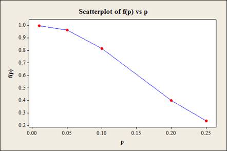
Sketch the OC curve for the accepting sampling plan.
Answer to Problem 58E
The probability that the batch will be accepted for different values of actual proportion of defectives,
| p | |
| 0.01 | 0.996 |
| 0.05 | 0.9638 |
| 0.1 | 0.8159 |
| 0.20 | 0.3980 |
| 0.25 | 0.2360 |
The OC curve is given below
Explanation of Solution
Given info:
10 is replaced by 15.
Calculation:
Let p be the actual proportion of defective in the batch.
Let X be the number of defectives in the sample.
The sample size is 15. The samples are selected randomly and the outcomes are defective or non-defective.
Hence,
It is given that the batch will be accepted if the number of defective components in the sample is at most 2 means the batch will be accepted if
The probability that the batch will be accepted when the actual proportion of defectives is p, is
The probability values:
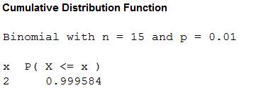
For p = 0.01:
Software procedure:
Step by step procedure to obtain the probability values using the MINITAB software:
- Choose Calc > Probability Distribution> Binomial Distribution.
- Enter number of trials as 15 and event probability as 0.01
- Choose Cumulative probability.
- In Input constant, enter 2.
- Click OK.
Output using MINITAB software is given below:
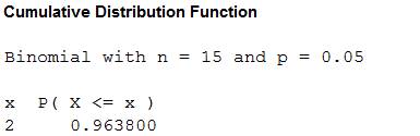
For p = 0.05:
Software procedure:
Step by step procedure to obtain the probability values using the MINITAB software:
- Choose Calc > Probability Distribution> Binomial Distribution.
- Enter number of trials as 15 and event probability as 0.05
- Choose Cumulative probability.
- In Input constant, enter 2.
- Click OK.
Output using MINITAB software is given below:
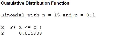
For p = 0.10:
Software procedure:
Step by step procedure to obtain the probability values using the MINITAB software:
- Choose Calc > Probability Distribution> Binomial Distribution.
- Enter number of trials as 15 and event probability as 0.10
- Choose Cumulative probability.
- In Input constant, enter 2.
- Click OK.
Output using MINITAB software is given below:
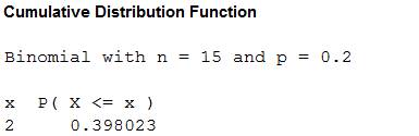
For p = 0.2:
Software procedure:
Step by step procedure to obtain the probability values using the MINITAB software:
- Choose Calc > Probability Distribution> Binomial Distribution.
- Enter number of trials as 15 and event probability as 0.20
- Choose Cumulative probability.
- In Input constant, enter 2.
- Click OK.
Output using MINITAB software is given below:
For p = 0.25:
Software procedure:
Step by step procedure to obtain the probability values using the MINITAB software:
- Choose Calc > Probability Distribution> Binomial Distribution.
- Enter number of trials as 15 and event probability as 0.25
- Choose Cumulative probability.
- In Input constant, enter 2.
- Click OK.
Output using MINITAB software is given below:
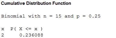
Hence, the probability that the batch will be accepted for different values of actual proportion of defectives,
| p | |
| 0.01 | 0.996 |
| 0.05 | 0.9638 |
| 0.1 | 0.8159 |
| 0.20 | 0.3980 |
| 0.25 | 0.2360 |
OC curve:
Software procedure:
Step by step procedure to obtain the probability values using the MINITAB software:
- Choose Graph > Scatterplot.
- Choose With Connect Line, and then click OK.
- Under Y variables, enter a column of f(p).
- Under X variables, enter a column of p.
- Click OK.
Output using MINITAB software is given below:
e.
Find the most satisfactory sampling plan among a, c and d.
Answer to Problem 58E
Plan in part (d) is most satisfactory.
Explanation of Solution
Justification:
It is known that a batch is characterized as acceptable if the proportion of defective components is at most 0.10 that is
Hence, the desirable probability of accepting a batch should be high when
Comparing the three sampling plan, it can be observed that for p = 0.25, the probability of accepting a batch is lowest for sampling plan in part (d) and for p = 0.01, the probability of accepting a batch is highest for sampling plan in part (d).
Hence, the sampling plan in part (d) is most satisfactory.
Want to see more full solutions like this?
Chapter 3 Solutions
EBK PROBABILITY AND STATISTICS FOR ENGI


- F Make a box plot from the five-number summary: 100, 105, 120, 135, 140. harrow_forward14 Is the standard deviation affected by skewed data? If so, how? foldarrow_forwardFrequency 15 Suppose that your friend believes his gambling partner plays with a loaded die (not fair). He shows you a graph of the outcomes of the games played with this die (see the following figure). Based on this graph, do you agree with this person? Why or why not? 65 Single Die Outcomes: Graph 1 60 55 50 45 40 1 2 3 4 Outcome 55 6arrow_forward
- lie y H 16 The first month's telephone bills for new customers of a certain phone company are shown in the following figure. The histogram showing the bills is misleading, however. Explain why, and suggest a solution. Frequency 140 120 100 80 60 40 20 0 0 20 40 60 80 Telephone Bill ($) 100 120arrow_forward25 ptical rule applies because t Does the empirical rule apply to the data set shown in the following figure? Explain. 2 6 5 Frequency 3 сл 2 1 0 2 4 6 8 00arrow_forward24 Line graphs typically connect the dots that represent the data values over time. If the time increments between the dots are large, explain why the line graph can be somewhat misleading.arrow_forward
- 17 Make a box plot from the five-number summary: 3, 4, 7, 16, 17. 992) waarrow_forward12 10 - 8 6 4 29 0 Interpret the shape, center and spread of the following box plot. brill smo slob.nl bagharrow_forwardSuppose that a driver's test has a mean score of 7 (out of 10 points) and standard deviation 0.5. a. Explain why you can reasonably assume that the data set of the test scores is mound-shaped. b. For the drivers taking this particular test, where should 68 percent of them score? c. Where should 95 percent of them score? d. Where should 99.7 percent of them score? Sarrow_forward
- 13 Can the mean of a data set be higher than most of the values in the set? If so, how? Can the median of a set be higher than most of the values? If so, how? srit to estaarrow_forwardA random variable X takes values 0 and 1 with probabilities q and p, respectively, with q+p=1. find the moment generating function of X and show that all the moments about the origin equal p. (Note- Please include as much detailed solution/steps in the solution to understand, Thank you!)arrow_forward1 (Expected Shortfall) Suppose the price of an asset Pt follows a normal random walk, i.e., Pt = Po+r₁ + ... + rt with r₁, r2,... being IID N(μ, o²). Po+r1+. ⚫ Suppose the VaR of rt is VaRq(rt) at level q, find the VaR of the price in T days, i.e., VaRq(Pt – Pt–T). - • If ESq(rt) = A, find ES₁(Pt – Pt–T).arrow_forward

 Holt Mcdougal Larson Pre-algebra: Student Edition...AlgebraISBN:9780547587776Author:HOLT MCDOUGALPublisher:HOLT MCDOUGAL
 College Algebra (MindTap Course List)AlgebraISBN:9781305652231Author:R. David Gustafson, Jeff HughesPublisher:Cengage Learning
 Algebra and Trigonometry (MindTap Course List)AlgebraISBN:9781305071742Author:James Stewart, Lothar Redlin, Saleem WatsonPublisher:Cengage Learning
 College AlgebraAlgebraISBN:9781305115545Author:James Stewart, Lothar Redlin, Saleem WatsonPublisher:Cengage Learning
 Algebra & Trigonometry with Analytic GeometryAlgebraISBN:9781133382119Author:SwokowskiPublisher:Cengage