Videos
Size of Dams These data represent the volumes in cubic yards of the largest dams in the United States and in South America. Construct a boxplot of the data for each region and compare the distributions.
| United States | South America |
| 125,628 92,000 78,008 77,700 66,500 62,850 52,435 50,000 |
311,539 274,026 105,944 102,014 56,242 46,563 |
The boxplot of the given data and comparison of the distribution.
Answer to Problem 16E
The boxplot for the capacity of dams in the United States is shown below,
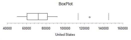
Fig (1)
The boxplot for the capacity of dams in the South America is shown below,
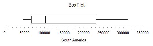
Fig (2)
The range and variation of the capacity of the dams in South America is larger than the capacity of the dams in United Stated.
Explanation of Solution
Given info:
The data of the capacity of dams in the United States and the South America is shown in the table below.
| United States | South America |
| 125628 | 311539 |
| 92000 | 274026 |
| 78008 | 105944 |
| 77700 | 102014 |
| 66500 | 56242 |
| 62850 | 46563 |
| 52435 | |
| 50000 |
Calculation:
The boxplot is used to graphically depict groups of numerical data through their quantities.
Arrange the densities of dams in the United States in ascending order as shown below.
| United States |
| 50000 |
| 52435 |
| 62850 |
| 66500 |
| 77700 |
| 78008 |
| 92000 |
| 125628 |
The minimum capacity of the dam from the above table is 50000 and the maximum capacity of the dam is 125628.
The number of data in the table is 8.
The formula to calculate the median for even data is shown below.
The total number of terms in the data is 8 so, substitute 8 for n in the above formula.
Substitute 66500 for
Thus, the median of the data is 72,100.
Software procedure:
Step-by-step procedure to construct boxplot by using Excel add-in (MegaStat).
- First select the data for which boxplot is obtained.
- Click on Add-Ins option in the top.
- Click on MegaStat option on the left side of the screen and then click on descriptive statistics.
- Select the boxplot option then in input range, select the data cells and then click ok.
Observation:
Since median falls to the right of the centre of the box thus the distribution is slightly negatively skewed.
Now, arrange the data of densities of dams in the South America in ascending order as shown below.
| South America |
| 46563 |
| 56242 |
| 102014 |
| 105944 |
| 274026 |
| 311539 |
The minimum capacity of the dam from the above table is 46563 and the maximum capacity of the dam is 311539.
The number of data in the table is 6.
The formula to calculate the median for even data is shown below.
The total number of terms in the data is 6 so, substitute 6 for n in the above formula.
Substitute 102014 for
Thus, the median of the data is 103,979.
Software procedure:
Step-by-step procedure to construct boxplot by using Excel add-in (MegaStat).
- First select the data for which boxplot is obtained.
- Click on Add-Ins option in the top.
- Click on MegaStat option on the left side of the screen and then click on descriptive statistics.
- Select the boxplot option then in input range, select the data cells and then click ok.
Observation:
Since median falls to the left of the centre of the box thus the distribution is slightly positively skewed.
The range and variation of the capacity of the dams in South America is larger than the capacity of the dams in United Stated.
Want to see more full solutions like this?
Chapter 3 Solutions
Elementary Statistics: A Step-by-Step Approach with Formula Card


- Examine the Variables: Carefully review and note the names of all variables in the dataset. Examples of these variables include: Mileage (mpg) Number of Cylinders (cyl) Displacement (disp) Horsepower (hp) Research: Google to understand these variables. Statistical Analysis: Select mpg variable, and perform the following statistical tests. Once you are done with these tests using mpg variable, repeat the same with hp Mean Median First Quartile (Q1) Second Quartile (Q2) Third Quartile (Q3) Fourth Quartile (Q4) 10th Percentile 70th Percentile Skewness Kurtosis Document Your Results: In RStudio: Before running each statistical test, provide a heading in the format shown at the bottom. “# Mean of mileage – Your name’s command” In Microsoft Word: Once you've completed all tests, take a screenshot of your results in RStudio and paste it into a Microsoft Word document. Make sure that snapshots are very clear. You will need multiple snapshots. Also transfer these results to the…arrow_forward2 (VaR and ES) Suppose X1 are independent. Prove that ~ Unif[-0.5, 0.5] and X2 VaRa (X1X2) < VaRa(X1) + VaRa (X2). ~ Unif[-0.5, 0.5]arrow_forward8 (Correlation and Diversification) Assume we have two stocks, A and B, show that a particular combination of the two stocks produce a risk-free portfolio when the correlation between the return of A and B is -1.arrow_forward
- 9 (Portfolio allocation) Suppose R₁ and R2 are returns of 2 assets and with expected return and variance respectively r₁ and 72 and variance-covariance σ2, 0%½ and σ12. Find −∞ ≤ w ≤ ∞ such that the portfolio wR₁ + (1 - w) R₂ has the smallest risk.arrow_forward7 (Multivariate random variable) Suppose X, €1, €2, €3 are IID N(0, 1) and Y2 Y₁ = 0.2 0.8X + €1, Y₂ = 0.3 +0.7X+ €2, Y3 = 0.2 + 0.9X + €3. = (In models like this, X is called the common factors of Y₁, Y₂, Y3.) Y = (Y1, Y2, Y3). (a) Find E(Y) and cov(Y). (b) What can you observe from cov(Y). Writearrow_forward1 (VaR and ES) Suppose X ~ f(x) with 1+x, if 0> x > −1 f(x) = 1−x if 1 x > 0 Find VaRo.05 (X) and ES0.05 (X).arrow_forward
- Joy is making Christmas gifts. She has 6 1/12 feet of yarn and will need 4 1/4 to complete our project. How much yarn will she have left over compute this solution in two different ways arrow_forwardSolve for X. Explain each step. 2^2x • 2^-4=8arrow_forwardOne hundred people were surveyed, and one question pertained to their educational background. The results of this question and their genders are given in the following table. Female (F) Male (F′) Total College degree (D) 30 20 50 No college degree (D′) 30 20 50 Total 60 40 100 If a person is selected at random from those surveyed, find the probability of each of the following events.1. The person is female or has a college degree. Answer: equation editor Equation Editor 2. The person is male or does not have a college degree. Answer: equation editor Equation Editor 3. The person is female or does not have a college degree.arrow_forward
 Glencoe Algebra 1, Student Edition, 9780079039897...AlgebraISBN:9780079039897Author:CarterPublisher:McGraw Hill
 Holt Mcdougal Larson Pre-algebra: Student Edition...AlgebraISBN:9780547587776Author:HOLT MCDOUGALPublisher:HOLT MCDOUGAL
 Big Ideas Math A Bridge To Success Algebra 1: Stu...AlgebraISBN:9781680331141Author:HOUGHTON MIFFLIN HARCOURTPublisher:Houghton Mifflin Harcourt
 Algebra: Structure And Method, Book 1AlgebraISBN:9780395977224Author:Richard G. Brown, Mary P. Dolciani, Robert H. Sorgenfrey, William L. ColePublisher:McDougal Littell