
Subpart (a):
Long run equilibrium in AD-AS model.
Subpart (a):
Explanation of Solution
The supply depends upon the
The demand comes from all the economic agents such as the households, firms as well as the government. The demand depends on the price level of the economy. The increase and decrease in the price level determines the level of demand in the economy. The aggregation of all the individual demands in the economy is known as the aggregate demand thus, the aggregate demand explains the relationship between the general price level and the level of real
The equilibrium is a condition where the aggregate demand curve of the economy intersects with the aggregate supply curve of the economy. Then there will be an equilibrium point derived where the economy will be in its equilibrium without any excess demand or supply. The quantity on the X axis will represent the
Concept introduction:
Aggregate demand curve: It is the curve which shows the relationship between the price level in the economy and the quantity of real GDP demanded by the economic agents such as the households, firms as well as the government.
Equilibrium: The equilibrium in the economy is the point where the economy's aggregate demand curve and the aggregate supply curve intersects with each other. There will be no excess demand or
Subpart (b):
Long run equilibrium in AD-AS model.
Subpart (b):
Explanation of Solution
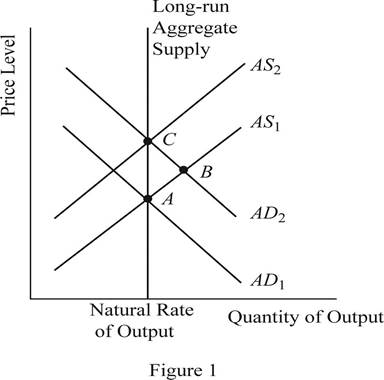
When the money supply of the economy increases with the intervention of the Central Bank of the economy, the money with the public will increase. When the money with the public increases, they will feel wealthier and as a result they will demand more consumer goods and services. As a result, the aggregate demand of the economy increases and it will shift the AD curve towards the right. This can be identified as the change to the equilibrium point B as shown in Figure 1. Thus, in short, the increase in the money supply leads to the increase in the output and price level of the economy.
Concept introduction:
Aggregate demand curve: It is the curve which shows the relationship between the price level in the economy and the quantity of real GDP demanded by the economic agents such as the households, firms as well as the government.
Aggregate supply curve: In the short run, it is a curve which shows the relationship between the price level in the economy and the supply in the economy by the firms. In the long run, it shows the relationship between the price level and the level of quantity supplied by the firms.
Equilibrium: The equilibrium in the economy is the point where the economy's aggregate demand curve and the aggregate supply curve intersects with each other. There will be no excess demand or excess supply in the economy at the equilibrium.
Subpart (c):
Long run equilibrium in AD-AS model.
Subpart (c):
Explanation of Solution
When the AD curve shifts towards the right and increases the output and the price level in the short run, over time, the nominal wages, prices as well as the perceptions and expectations of the economy would adjust to the new equilibrium level. As a result of this gradual adjustment, the cost of production will increase and the result will be a leftward shift in the aggregate supply curve of the economy. Then the economy will return to its natural level of output at a higher price level of the economy. This can be identified as the movement from point B to point C in the graph shown above.
Concept introduction:
Aggregate demand curve: It is the curve which shows the relationship between the price level in the economy and the quantity of real GDP demanded by the economic agents such as the households, firms as well as the government.
Aggregate supply curve: In the short run, it is a curve which shows the relationship between the price level in the economy and the supply in the economy by the firms. In the long run, it shows the relationship between the price level and the level of quantity supplied by the firms.
Equilibrium: The equilibrium in the economy is the point where the economy's aggregate demand curve and the aggregate supply curve intersects with each other. There will be no excess demand or excess supply in the economy at the equilibrium.
Subpart (d):
Long run equilibrium in AD-AS model.
Subpart (d):
Explanation of Solution
The sticky wages theory suggests that when there is inflation in the economy, the wage rate will adjust very slowly to the inflation. More or less the wage rates will be sticky and the main reason will be the long term contracts between the employer and the employees. Thus, in the short run equilibriums such as point A and point B, the wages of the economy would be more or less equal to each other. Whereas the point C represents the long run equilibrium and thus, the wages at the point C will be higher than that in point A and B.
Concept introduction:
Aggregate demand curve: It is the curve which shows the relationship between the price level in the economy and the quantity of real GDP demanded by the economic agents such as the households, firms as well as the government.
Aggregate supply curve: In the short run, it is a curve which shows the relationship between the price level in the economy and the supply in the economy by the firms. In the long run, it shows the relationship between the price level and the level of quantity supplied by the firms.
Equilibrium: The equilibrium in the economy is the point where the economy's aggregate demand curve and the aggregate supply curve intersects with each other. There will be no excess demand or excess supply in the economy at the equilibrium.
Subpart (e):
Long run equilibrium in AD-AS model.
Subpart (e):
Explanation of Solution
The sticky wages theory suggests that when there is inflation in the economy, the wage rate will adjust very slowly to the inflation. More or less, the wage rates will be sticky and the main reason will be the long term contracts between the employer and the employees. So, the nominal wages at equilibrium point A and B will be same. But the increase in the general price level in the economy would reduce the real wages of the workers because, the real wage is the nominal wage divided by the price level. When the denominator increases, it will reduce the value of the real wages in the economy.
Concept introduction:
Aggregate demand curve: It is the curve which shows the relationship between the price level in the economy and the quantity of real GDP demanded by the economic agents such as the households, firms as well as the government.
Aggregate supply curve: In the short run, it is a curve which shows the relationship between the price level in the economy and the supply in the economy by the firms. In the long run, it shows the relationship between the price level and the level of quantity supplied by the firms.
Equilibrium: The equilibrium in the economy is the point where the economy's aggregate demand curve and the aggregate supply curve intersects with each other. There will be no excess demand or excess supply in the economy at the equilibrium.
Sub part (f):
Long run equilibrium in AD-AS model.
Sub part (f):
Explanation of Solution
When the increase in the money supply happens in the economy, it will lead to the increase in the nominal wages as well as the price level in the economy in the long run. As a result of the increase in the nominal wage rate along with the price level in the economy, the real wage rate of the economy would remain unchanged. Thus, the neutrality of money applies in the long run equilibrium.
Concept introduction:
Aggregate demand curve: It is the curve which shows the relationship between the price level in the economy and the quantity of real GDP demanded by the economic agents such as the households, firms as well as the government.
Aggregate supply curve: In the short run, it is a curve which shows the relationship between the price level in the economy and the supply in the economy by the firms. In the long run, it shows the relationship between the price level and the level of quantity supplied by the firms.
Equilibrium: The equilibrium in the economy is the point where the economy's aggregate demand curve and the aggregate supply curve intersects with each other. There will be no excess demand or excess supply in the economy at the equilibrium.
Want to see more full solutions like this?
Chapter 33 Solutions
MindTap Economics, 2 terms (12 months) Printed Access Card for Mankiw's Principles of Economics, 8th (MindTap Course List)

- Question 1 Coursology Consider the four policies bellow. Classify them as either fiscal or monetary policy: I. The United States Government promoting tax cuts for small businesses to prevent a wave of bankruptcies during the COVID-19 pandemic II. The Congress approving a higher budget for the Affordable Health Care Act (also known as Obamacare) III. The Federal Reserve increasing the required reserves for commercial banks aiming to control the rise of inflation IV. President Joe Biden approving a new round of stimulus checks for households I. fiscal, II. fiscal, III. monetary, IV. fiscal I. fiscal, II. monetary, III. monetary, IV. monetary I. monetary, II. fiscal, III. fiscal, IV. fiscal I. monetary, II. monetary, III. fiscal, IV. monetaryarrow_forwardConsider the following supply and demand schedule of wooden tables.a. Draw the corresponding graphs for supply and demand.b. Using the data, obtain the corresponding supply and demand functions. c. Find the market-clearing price and quantity. Price (Thousand s USD Supply Demand 2 96 1104 196 1906 296 2708 396 35010 496 43012 596 51014 696 59016 796 67018 896 75020…arrow_forwardConsider a firm with the following production function Q=5000L-2L2.a. Find the maximum production level.b. How many units of labour are needed at that point. c. Obtain the function of marginal product of labour (MRL) d. Graph the production function and the MRL.arrow_forward
- Exercise 4A firm has the following total cost function TC=100q-5q2+0.5q3. Find the average cost function.arrow_forwardA firm has the following demand function P=200 − 2Q and the average costof AC= 100/Q + 3Q −20.a. Find the profit function. b. Estimate the marginal cost function. c. Obtain the production that maximizes the profit. d. Evaluate the average cost and the marginal cost at the maximising production level.arrow_forwardRubber: Initial investment: $159,000 Annual cost: $36,000 Annual revenue: $101,000 Salvage value: $12,000 Useful life: 10 years Using the cotermination assumptions, a study period of 6 years, and a MARR of 9%, what is the present worth of the rubber alternative? Assume that the rubber alternative's equipment has a market value of $18,000 at the end of Year 6.arrow_forward
- Richard has just opened a new restaurant. Not being good at deserts, he has contracted with Carla to provide pies. Carla’s costs are $10 per pie, and she sells the pies to Richard for $25 each. Richard resells them for $50, and he incurs no costs other than the $25 he pays Carla. Assume Carla’s costs go up to $30 per pie. If courts always award expectation damages, which of the following statements is most likely to be true?arrow_forwardDifference-in-Difference In the beginning of 2001, North Dakota legalized fireworks. Suppose you are interested in studying the effect of the legalizing of fireworks on the number of house fires in North Dakota. Unlike North Dakota, South Dakota did not legalize fireworks and continued to ban them. You decide to use a Difference-in-difference (DID) Model. The numbers of house fires in each state at the end of 2000 and 2001 are as follows: Number of house fires in Number of house fires in Year North Dakota 2000 2001 35 50 South Dakota 54 64 a. What is the change in the outcome for the treatment group between 2000 and 2001? Show your working for full credit. (10 points) b. Can we interpret the change in the outcome for the treatment group between 2000 and 2001 as the causal effect of legalizing fireworks on number of house fires? Explain your answer. (10 points)arrow_forwardC. Regression Discontinuity Birth weight is used as a common sign for a newborn's health. In the United States, if a baby has a birthweight below 1500 grams, the newborn is classified as having “very low birth weight". Suppose you want to study the effect of having very low birth weight on the number of hospital visits made before the baby's first birthday. You decide to use Regression Discontinuity to answer this question. The graph below shows the RD model: Number of hospital visits made before baby's first birthday 5 1400 1450 1500 1550 1600 Birthweight (in grams) a. What is the running variable? (5 points) b. What is the cutoff? (5 points) T What is the discontinuity in the graph and how do you interpret it? (10 points)arrow_forward
- C. Regression Discontinuity Birth weight is used as a common sign for a newborn's health. In the United States, if a baby has a birthweight below 1500 grams, the newborn is classified as having “very low birth weight". Suppose you want to study the effect of having very low birth weight on the number of hospital visits made before the baby's first birthday. You decide to use Regression Discontinuity to answer this question. The graph below shows the RD model: Number of hospital visits made before baby's first birthday 5 1400 1450 1500 1550 1600 Birthweight (in grams) a. What is the running variable? (5 points) b. What is the cutoff? (5 points) T What is the discontinuity in the graph and how do you interpret it? (10 points)arrow_forwardExperiments Research suggests that if students use laptops in class, it can have some effect on student achievement. While laptop usage can help students take lecture notes faster, some argue that the laptops may be a source of distraction for the students. Suppose you are interested in looking at the effect of using laptops in class on the students' final exam scores out of 100. You decide to conduct a randomized control trial where you randomly assign some students at UIC to use a laptop in class and other to not use a laptop in class. (Assume that the classes are in person and not online) a. Which people are a part of the treatment group and which people are a part of the control group? (10 points) b. What regression will you run? Define the variables where required. (10 points)arrow_forwardExperiments Research suggests that if students use laptops in class, it can have some effect on student achievement. While laptop usage can help students take lecture notes faster, some argue that the laptops may be a source of distraction for the students. Suppose you are interested in looking at the effect of using laptops in class on the students' final exam scores out of 100. You decide to conduct a randomized control trial where you randomly assign some students at UIC to use a laptop in class and other to not use a laptop in class. (Assume that the classes are in person and not online) a. Which people are a part of the treatment group and which people are a part of the control group? (10 points) b. What regression will you run? Define the variables where required. (10 points)arrow_forward
 Essentials of Economics (MindTap Course List)EconomicsISBN:9781337091992Author:N. Gregory MankiwPublisher:Cengage Learning
 Principles of Economics (MindTap Course List)EconomicsISBN:9781305585126Author:N. Gregory MankiwPublisher:Cengage Learning
 Principles of Macroeconomics (MindTap Course List)EconomicsISBN:9781285165912Author:N. Gregory MankiwPublisher:Cengage Learning
 Brief Principles of Macroeconomics (MindTap Cours...EconomicsISBN:9781337091985Author:N. Gregory MankiwPublisher:Cengage Learning
 Principles of Economics, 7th Edition (MindTap Cou...EconomicsISBN:9781285165875Author:N. Gregory MankiwPublisher:Cengage Learning
 Principles of Macroeconomics (MindTap Course List)EconomicsISBN:9781305971509Author:N. Gregory MankiwPublisher:Cengage Learning