
Sub part (a):
Consumption schedule and marginal propensity to consume.
Sub part (a):
Explanation of Solution
Table -1 shows the consumption schedule:
Table -1
| Consumption | |
| 100 | 120 |
| 200 | 200 |
| 300 | 280 |
| 400 | 360 |
| 500 | 440 |
| 600 | 520 |
| 700 | 600 |
Figure 1 illustrates the level of consumption at different level of gross domestic product (GDP).
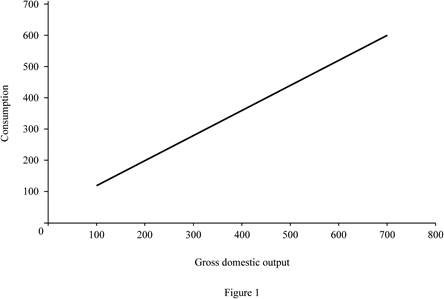
In Figure 1, the horizontal axis measures the gross domestic output and the vertical axis measures the consumption level.
Size of marginal propensity to consume (MPC) can be calculated as follows.
The size of marginal propensity to consume is 0.8.
Concept introduction:
Consumption schedule: Consumption schedule refers to the quantity of consumption at different levels of income.
Marginal propensity to consume (MPS): Marginal propensity to consume refers to the sensitivity of change in the consumption level due to the changes occurred in the income level.
Sub part (b):
Disposable income, tax rate, consumption schedule, marginal propensity to consume and multiplier.
Sub part (b):
Explanation of Solution
Disposable income (DI) can be calculated by using the following formula.
Substitute the respective values in Equation (1) to calculate the disposable income at the level of GDP $100.
Disposable income at the level of GDP $100 is $90.
Tax rate can be calculated by using the following formula.
Substitute the respective values in Equation (2) to calculate the tax rate at the level of GDP $100.
Tax rate at the level of GDP is 10%.
New consumption level can be calculated by using the following formula.
Substitute the respective values in Equation (3) to calculate the disposable income at the level of GDP $100. Since, the tax payment is equal amount of decrease in consumption for all the levels of GDP. The decreasing consumption for increasing $10 is assumed to be $8.
New consumption is $112.
Table -2 shows the values of disposable income, new consumption level after tax and the tax rate that are obtained by using Equations (1), (2) and (3).
Table -2
| Gross domestic product | Tax | DI | New consumption | Tax rate |
| 100 | 10 | 90 | 112 | 10% |
| 200 | 10 | 190 | 192 | 5% |
| 300 | 10 | 290 | 272 | 3.33% |
| 400 | 10 | 390 | 352 | 2.5% |
| 500 | 10 | 490 | 432 | 2% |
| 600 | 10 | 590 | 512 | 1.67% |
| 700 | 10 | 690 | 592 | 1.43% |
Size of marginal propensity to consume (MPC) can be calculated as follows.
The size of marginal propensity to consume is 0.8.
Multiplier: Multiplier refers to the ratio of change in the real GDP to the change in initial consumption, at a constant price rate. Multiplier is positively related to the marginal propensity to consumer and negatively related with the marginal propensity to save. Multiplier can be evaluated using the following formula:
Since the value of MPC remains the same for part (a) and part (b), there is no change in the value of multiplier. The value of multiplier is 5
Figure -2 illustrates the level of consumption at different level of gross domestic product (GDP) for lump sum tax (Regressive tax).
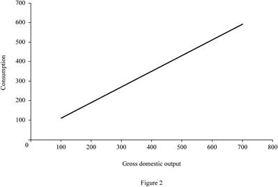
In Figure -2, the horizontal axis measures the gross domestic output and the vertical axis measures the consumption level.
Concept introduction:
Consumption schedule: Consumption schedule refers to the quantity of consumption at different levels of income.
Marginal propensity to consume (MPS): Marginal propensity to consume refers to the sensitivity of change in the consumption level due to the changes occurred in the income level.
Multiplier: Multiplier refers to the ratio of change in the real GDP to the change in initial consumption at constant price rate. Multiplier is positively related to the marginal propensity to consumer and negatively related with the marginal propensity to save.
Sub part (c):
Tax amount, consumption schedule, marginal propensity to consume and multiplier.
Sub part (c):
Explanation of Solution
Tax amount can be calculated by using the following formula.
Substitute the respective values in Equation (4) to calculate the tax amount at $100 GDP.
Tax amount is $10.
Table -3 shows the values of disposable income, new consumption level after tax and the tax rate that are obtained by using Equations (1), (2), (3) and (4). The change in tax amount is differing for different levels of GDP. The decreasing consumption for increasing each $10 is assumed to be $8 (Thus, if the tax payment is $30, then the consumption decreases by $24
Table -3
| Gross domestic product | Tax | DI | New consumption | Tax rate |
| 100 | 10 | 90 | 112 | 10% |
| 200 | 20 | 180 | 184 | 10% |
| 300 | 30 | 270 | 256 | 10% |
| 400 | 40 | 360 | 328 | 10% |
| 500 | 50 | 450 | 400 | 10% |
| 600 | 60 | 540 | 472 | 10% |
| 700 | 70 | 630 | 544 | 10% |
Multiplier: Multiplier refers to the ratio of change in the real GDP to the change in initial consumption, at a constant price rate. Multiplier is positively related to the marginal propensity to consumer and negatively related with the marginal propensity to save. Multiplier can be evaluated using the following formula:
Since the value of MPC different for part (a) and part (c), the value of multiplier for both the part is different. The value of multiplier is 3.57
Figure -3 illustrates the level of consumption at different level of gross domestic product (GDP) for proportional tax.
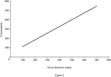
In Figure -3, the horizontal axis measures the gross domestic output and the vertical axis measures the consumption level.
Concept introduction:
Consumption schedule: Consumption schedule refers to the quantity of consumption at different levels of income.
Marginal propensity to consume (MPS): Marginal propensity to consume refers to the sensitivity of change in the consumption level due to the changes occurred in the income level.
Multiplier: Multiplier refers to the ratio of change in the real GDP to the change in initial consumption at constant price rate. Multiplier is positively related to the marginal propensity to consumer and negatively related with the marginal propensity to save.
Sub part (d):
consumption schedule, marginal propensity to consume and multiplier.
Sub part (d):
Explanation of Solution
Marginal propensity to consume can be calculated by using the following formula.
Substitute the respective values in Equation (5) to calculate the MPC at $100 GDP.
The value of MPC is 0.72.
Table -4 shows the values of disposable income, new consumption level after tax and the tax rate that are obtained by using Equations (1), (2), (3), (4) and (5). The change in tax amount is differing for different levels of GDP. The decreasing consumption for increasing each $10 is assumed to be $8 (Thus, if the tax payment is $20, then the consumption decreases by $16
Table -3
| Gross domestic product | Tax | DI | New consumption | Tax rate | MPC |
| 100 | 0 | 100 | 120 | 0% | |
| 200 | 10 | 190 | 192 | 5% | 0.8 |
| 300 | 30 | 270 | 256 | 10% | 0.64 |
| 400 | 60 | 340 | 312 | 15% | 0.56 |
| 500 | 100 | 400 | 360 | 20% | 0.48 |
| 600 | 150 | 450 | 400 | 25% | 0.4 |
| 700 | 210 | 490 | 432 | 30% | 0.32 |
Multiplier: Multiplier refers to the ratio of change in the real GDP to the change in initial consumption, at a constant price rate. Multiplier is positively related to the marginal propensity to consumer and negatively related with the marginal propensity to save.
Multiplier value is differing for each level of GDP. When the tax rate increases, it reduces the value of MPC. Since the value of MPC decreases, the value of multiplier will also decrease.
Figure 4 illustrates the level of consumption at different level of gross domestic product (GDP) for progressive tax.
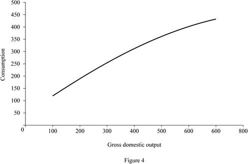
In Figure 4, the horizontal axis measures the gross domestic output and the vertical axis measures the consumption level.
Concept introduction:
Consumption schedule: Consumption schedule refers to the quantity of consumption at different levels of income.
Marginal propensity to consume (MPS): Marginal propensity to consume refers to the sensitivity of change in the consumption level due to the changes occurred in the income level.
Multiplier: Multiplier refers to the ratio of change in the real GDP to the change in initial consumption at constant price rate. Multiplier is positively related to the marginal propensity to consumer and negatively related with the marginal propensity to save.
Sup part (e):
Marginal propensity to consume and multiplier.
Sup part (e):
Explanation of Solution
Figure 1, Figure 2, Figure 3 and Figure 4 reveals that the proportional and progressive tax system reduces the value of MPC, so that the value of multiplier also decreases. The regressive tax system (Lump sum tax) does not alter the MPC. Since there is no change in the MPC, the multiplier remains the same.
Concept introduction:
Marginal propensity to consume (MPS): Marginal propensity to consume refers to the sensitivity of change in the consumption level due to the changes occurred in the income level.
Progressive tax: Progressive tax refers to the higher income people paying higher tax amount than the lower income people.
Proportional tax: Proportional tax rate refers to the fixed tax rate regardless of income and the tax rate and is the same for all levels of income.
Regressive tax: Regressive tax refers to the higher income people paying lower percentage of tax amount and lower income people paying higher percentage of tax amount.
Multiplier: Multiplier refers to the ratio of change in the real GDP to the change in initial consumption at constant price rate. Multiplier is positively related to the marginal propensity to consumer and negatively related with the marginal propensity to save.
Want to see more full solutions like this?

- What are some of the question s that I can ask my economic teacher?arrow_forwardAnswer question 2 only.arrow_forward1. A pension fund manager is considering three mutual funds. The first is a stock fund, the second is a long-term government and corporate fund, and the third is a (riskless) T-bill money market fund that yields a rate of 8%. The probability distributions of the risky funds have the following characteristics: Standard Deviation (%) Expected return (%) Stock fund (Rs) 20 30 Bond fund (RB) 12 15 The correlation between the fund returns is .10.arrow_forward
- Frederick Jones operates a sole proprietorship business in Trinidad and Tobago. His gross annual revenue in 2023 was $2,000,000. He wants to register for VAT, but he is unsure of what VAT entails, the requirements for registration and what he needs to do to ensure that he is fully compliant with VAT regulations. Make reference to the Vat Act of Trinidad and Tobago and explain to Mr. Jones what VAT entails, the requirements for registration and the requirements to be fully compliant with VAT regulations.arrow_forwardCan you show me the answers for parts a and b? Thanks.arrow_forwardWhat are the answers for parts a and b? Thanksarrow_forward
- What are the answers for a,b,c,d? Are they supposed to be numerical answers or in terms of a variable?arrow_forwardSue is a sole proprietor of her own sewing business. Revenues are $150,000 per year and raw material (cloth, thread) costs are $130,000 per year. Sue pays herself a salary of $60,000 per year but gave up a job with a salary of $80,000 to run the business. ○ A. Her accounting profits are $0. Her economic profits are - $60,000. ○ B. Her accounting profits are $0. Her economic profits are - $40,000. ○ C. Her accounting profits are - $40,000. Her economic profits are - $60,000. ○ D. Her accounting profits are - $60,000. Her economic profits are -$40,000.arrow_forwardSelect a number that describes the type of firm organization indicated. Descriptions of Firm Organizations: 1. has one owner-manager who is personally responsible for all aspects of the business, including its debts 2. one type of partner takes part in managing the firm and is personally liable for the firm's actions and debts, and the other type of partner takes no part in the management of the firm and risks only the money that they have invested 3. owners are not personally responsible for anything that is done in the name of the firm 4. owned by the government but is usually under the direction of a more or less independent, state-appointed board 5. established with the explicit objective of providing goods or services but only in a manner that just covers its costs 6. has two or more joint owners, each of whom is personally responsible for all of the partnership's debts Type of Firm Organization a. limited partnership b. single proprietorship c. corporation Correct Numberarrow_forward
- The table below provides the total revenues and costs for a small landscaping company in a recent year. Total Revenues ($) 250,000 Total Costs ($) - wages and salaries 100,000 -risk-free return of 2% on owner's capital of $25,000 500 -interest on bank loan 1,000 - cost of supplies 27,000 - depreciation of capital equipment 8,000 - additional wages the owner could have earned in next best alternative 30,000 -risk premium of 4% on owner's capital of $25,000 1,000 The economic profits for this firm are ○ A. $83,000. B. $82,500. OC. $114,000. OD. $83,500. ○ E. $112,500.arrow_forwardOutput TFC ($) TVC ($) TC ($) (Q) 2 100 104 204 3 100 203 303 4 100 300 400 5 100 405 505 6 100 512 612 7 100 621 721 Given the information about short-run costs in the table above, we can conclude that the firm will minimize the average total cost of production when Q = (Round your response to the nearest whole number.)arrow_forwardThe following data show the total output for a firm when specified amounts of labour are combined with a fixed amount of capital. Assume that the wage per unit of labour is $20 and the cost of the capital is $100. Labour per unit of time 0 1 Total Output 0 25 T 2 3 4 5 75 137 212 267 The marginal product of labour is at its maximum when the firm changes the amount of labour hired from ○ A. 0 to 1 unit. ○ B. 3 to 4 units. OC. 2 to 3 units. OD. 1 to 2 units. ○ E. 4 to 5 units.arrow_forward
 Principles of Economics 2eEconomicsISBN:9781947172364Author:Steven A. Greenlaw; David ShapiroPublisher:OpenStax
 Principles of Economics (MindTap Course List)EconomicsISBN:9781305585126Author:N. Gregory MankiwPublisher:Cengage Learning
 Principles of Macroeconomics (MindTap Course List)EconomicsISBN:9781285165912Author:N. Gregory MankiwPublisher:Cengage Learning
 Brief Principles of Macroeconomics (MindTap Cours...EconomicsISBN:9781337091985Author:N. Gregory MankiwPublisher:Cengage Learning
 Principles of Economics, 7th Edition (MindTap Cou...EconomicsISBN:9781285165875Author:N. Gregory MankiwPublisher:Cengage Learning