
Subpart (a):
Effect on Aggregate Demand and Supply.
Subpart (a):
Explanation of Solution
When consumers fear of an impending economic depression, their spending decline and they tend to save more. This leads to a decrease in AD curve. This can be explained by using figure 1.
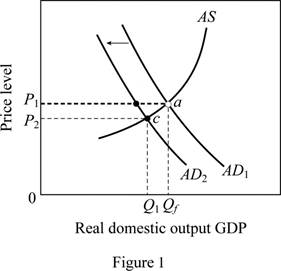
In figure 1, horizontal axis represents the real GDP(
Concept Introduction:
Aggregate demand (AD): Aggregate demand refers to the total value of the goods and services that are demanded at a particular price in a given period of time.
Subpart (b):
Effect on Aggregate Demand and Supply.
Subpart (b):
Explanation of Solution
When a new tax is imposed on producers, cost of production comes up and there is no incentive to produce more. This leads to a decline in
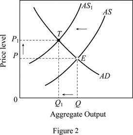
In figure 2, horizontal axis represents the real GDP and vertical axis represents price level. In this case, the AS curve shifts left (from AS to AS1), this moves the equilibrium position from E to T, thus there is a decline in the output (from Q to Q1) and a rise in the price level (from P to P1).
Concept Introduction:
Aggregate demand (AD): Aggregate demand refers to the total value of the goods and services that are demanded at a particular price in a given period of time.
Aggregate supply (AS): Aggregate supply refers to the total value of the goods and services that are available for purchase at a particular price in a given period of time.
Subpart (c):
Effect on Aggregate Demand and Supply.
Subpart (c):
Explanation of Solution
Figure 3 can explain the shift in AD curve due to reduction in interest rates at each price level. In figure 3, horizontal axis measures the real GDP and vertical axis measures the price level.
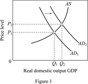
A reduction in interest rates decreases the borrowing cost increases the spending.
This leads to a rightward shift of AD curve from AD1 to AD2. Thus, it brings the output and price level up. The output increases from Q1 to Q2 and price level increases from P1 to P2.
Concept Introduction:
Aggregate demand (AD): Aggregate demand refers to the total value of the goods and services that are demanded at a particular price in a given period of time.
Aggregate supply (AS): Aggregate supply refers to the total value of the goods and services that are available for purchase at a particular price in a given period of time.
Subpart (d):
Effect on Aggregate Demand and Supply.
Subpart (d):
Explanation of Solution
A major increase in spending shifts the AD curve to right. Figure 4 is used to explain this situation. In figure 4, horizontal axis measures the real GDP and vertical axis measures the price level.
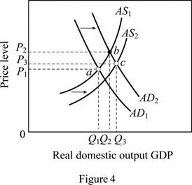
Government expenditure is a key determinant of changes in the aggregate demand. The increase in government spending (spending for health care) increases the aggregate demand leading to a shift of AD curve from AD1 to AD2. Any real improvements in healthcare resulting from the spending would ultimately increase the productivity, thereby shifting the AS curve to the right (from AS1 to AS2). The equilibrium moves from a to c leading to an increase in output (from Q1 to Q3) .It will also move the price level up from P1 to P3.
Concept Introduction:
Aggregate demand (AD): Aggregate demand refers to the total value of the goods and services that are demanded at a particular price in a given period of time.
Aggregate supply (AS): Aggregate supply refers to the total value of the goods and services that are available for purchase at a particular price in a given period of time.
Subpart (e):
Effect on Aggregate Demand and Supply.
Subpart (e):
Explanation of Solution
The general expectation of surging inflation in the near future will increase the aggregate demand today because the consumers will want to buy products before their prices escalate. This can be illustrated using figure 3. As a result, there will be a rightward shift of AD curve from AD1 to AD2 which brings the output and price level up. In figure 3, the output increases from Q1 to Q2 and price level increases from P1 to P2.
Concept Introduction:
Aggregate demand (AD): Aggregate demand refers to the total value of the goods and services that are demanded at a particular price in a given period of time.
Aggregate supply (AS): Aggregate supply refers to the total value of the goods and services that are available for purchase at a particular price in a given period of time.
Subpart (f):
Effect on Aggregate Demand and Supply.
Subpart (f):
Explanation of Solution
Figure 5 is used to explain this case. In figure 5, horizontal axis measures the real GDP and vertical axis measures the price level.
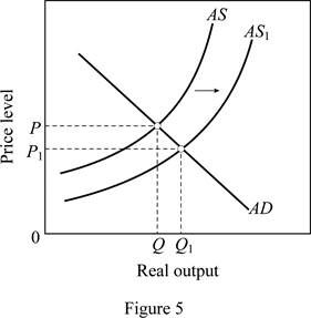
As oil prices fall (oil is an imported resource) due to the disintegration of OPEC, it increases the U.S. aggregate supply. As a result, there will be a rightward shift of AS curve from AS to AS1. This brings the output level up from Q to Q1 and price level down from P to P1.
Concept Introduction:
Aggregate demand (AD): Aggregate demand refers to the total value of the goods and services that are demanded at a particular price in a given period of time.
Aggregate supply (AS): Aggregate supply refers to the total value of the goods and services that are available for purchase at a particular price in a given period of time.
Subpart (g):
Effect on Aggregate Demand and Supply.
Subpart (g):
Explanation of Solution
A reduction in the personal income tax rates raises take-home income increases consumer purchases at each possible price level. This is illustrated in figure 3. Tax cuts shift the aggregate demand curve to the right from AD1 to AD2 which brings the output and price level up. In figure 3, the output increases from Q1 to Q2 and price level increases from P1 to P2.
Concept Introduction:
Aggregate demand (AD): Aggregate demand refers to the total value of the goods and services that are demanded at a particular price in a given period of time.
Aggregate supply (AS): Aggregate supply refers to the total value of the goods and services that are available for purchase at a particular price in a given period of time.
Subpart (h):
Effect on Aggregate Demand and Supply.
Subpart (h):
Explanation of Solution
The sizable increase the labor productivity with no change in nominal wages will increase the overall productivity as more output is available for the given input. This increases the aggregate supply thereby shifting the AS curve to the right from AS to AS1 (Refer Figure 5). This leads to an increase in output (from Q to Q1) and a decrease in price level from P to P1.
Concept Introduction:
Aggregate demand (AD): Aggregate demand refers to the total value of the goods and services that are demanded at a particular price in a given period of time.
Aggregate supply (AS): Aggregate supply refers to the total value of the goods and services that are available for purchase at a particular price in a given period of time.
Subpart (i):
Effect on Aggregate Demand and Supply.
Subpart (i):
Explanation of Solution
This case can be explained using Figure 2. When there is an increase in nominal wages with no change in productivity, it increases per unit cost of production. This force the AS curve to shift left (from AS to AS1). The equilibrium position moves from E to T, thus there are a decline in the output (from Q to Q1) and a rise in the price level (from P to P1).
Concept Introduction:
Aggregate demand (AD): Aggregate demand refers to the total value of the goods and services that are demanded at a particular price in a given period of time.
Aggregate supply (AS): Aggregate supply refers to the total value of the goods and services that are available for purchase at a particular price in a given period of time.
Subpart (j):
Effect on Aggregate Demand and Supply.
Subpart (j):
Explanation of Solution
Figure 6 shows the impact of increasing demand and decreasing supply.
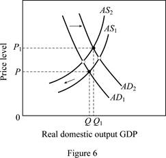
Figure 6 is used to explain this condition. The horizontal axis in Figure 6 measures the real domestic output whereas price level is measured by the vertical axis. A rise in net exports (higher exports relative to imports) shifts the aggregate demand curve to the right (from AD1 to AD2). But, due to the higher input prices, per unit cost is more, leading to a shift of the aggregate supply curve to the left from AS1 to AS2. This leads to an increase in output from Q to Q1 along with an increase in price level from P to P1.
Concept Introduction:
Aggregate demand (AD): Aggregate demand refers to the total value of the goods and services that are demanded at a particular price in a given period of time.
Aggregate supply (AS): Aggregate supply refers to the total value of the goods and services that are available for purchase at a particular price in a given period of time.
Want to see more full solutions like this?
Chapter 32 Solutions
Economics (Irwin Economics)

- 2. Answer the following questions as they relate to a fishery: Why is the maximum sustainable yield not necessarily the optimal sustainable yield? Does the same intuition apply to Nathaniel's decision of when to cut his trees? What condition will hold at the equilibrium level of fishing in an open-access fishery? Use a graph to explain your answer, and show the level of fishing effort. Would this same condition hold if there was only one boat in the fishery? If not, what condition will hold, and why is it different? Use the same graph to show the single boat's level of effort. Suppose you are given authority to solve the open-access problem in the fishery. What is the key problem that you must address with your policy?arrow_forward1. Repeated rounds of negotiation exacerbate the incentive to free-ride that exists for nations considering the ratification of international environmental agreements.arrow_forwardFor environmental Economics, A-C Pleasearrow_forward
- True/ False/ Undetermined - Environmental Economics 3. When the MAC is known but there is uncertainty about the MDF, an emissions quota leads to a lower deadweight loss associated with this uncertainty.arrow_forwardTrue/False/U- Environmental Economics 2. The discount rate used in climate integrated assessment models is the key driver of the intensity of emissions reductions associated with optimal climate policy in the model.arrow_forwardAt the beginning of the year, the market for portable electric fans was in equilibrium. In June, a summer heat wave hit. What effect does the heat wave have on the market for fans? Drag the appropriate part(s) of the graph to show the effect on the market for portable fans. To refer to the graphing tutorial for this question type, please click here. Price 17 OF 21 QUESTIONS COMPLETED f4 Q Search f5 f6 f7 CO hp fg 6 M366 W ins f12 f11 f10 SUBMIT ANSWER ENG 4xarrow_forward
- In the context of investment risk, what does "diversification" mean? A) Spreading investments across various assets to reduce riskB) Investing in a single asset to maximize returnsC) Increasing investment in high-risk assetsD) Reducing the number of investments to focus on high-performing onesarrow_forwardAt the 8:10 café, there are equal numbers of two types of customers with the following values. The café owner cannot distinguish between the two types of students because many students without early classes arrive early anyway (that is she cannot price discriminate). Students with early classes Students without early classes Coffee 70 60 Banana 50 100 The MC of coffee is 10. The MC of a banana is 40. Is bundling more profitable than selling separately? HINT: if you sell the bundle, can you make more by offering coffee separately? If so, what price should be charged for the bundle? (Show calculations)arrow_forwardYour marketing department has identified the following customer demographics in the following table. Construct a demand curve and determine the profit maximizing price as well as the expected profit if MC=$1. The number of customers in the target population is 10,000. Use the following demand data: Group Value Frequency Baby boomers $5 20% Generation X $4 10% Generation Y $3 10% `Tweeners $2 10% Seniors $2 10% Others $0 40%arrow_forward
- Your marketing department has identified the following customer demographics in the following table. Construct a demand curve and determine the profit maximizing price as well as the expected profit if MC=$1. The number of customers in the target population is 10,000. Group Value Frequency Baby boomers $5 20% Generation X $4 10% Generation Y $3 10% `Tweeners $2 10% Seniors $2 10% Others $0 40% ur marketing department has identified the following customer demographics in the following table. Construct a demand curve and determine the profit maximizing price as well as the expected profit if MC=$1. The number of customers in the target population is 10,000.arrow_forwardTest Preparation QUESTION 2 [20] 2.1 Body Mass Index (BMI) is a summary measure of relative health. It is calculated by dividing an individual's weight (in kilograms) by the square of their height (in meters). A small sample was drawn from the population of UWC students to determine the effect of exercise on BMI score. Given the following table, find the constant and slope parameters of the sample regression function of BMI = f(Weekly exercise hours). Interpret the two estimated parameter values. X (Weekly exercise hours) Y (Body-Mass index) QUESTION 3 2 4 6 8 10 12 41 38 33 27 23 19 Derek investigates the relationship between the days (per year) absent from work (ABSENT) and the number of years taken for the worker to be promoted (PROMOTION). He interviewed a sample of 22 employees in Cape Town to obtain information on ABSENT (X) and PROMOTION (Y), and derived the following: ΣΧ ΣΥ 341 ΣΧΥ 176 ΣΧ 1187 1012 3.1 By using the OLS method, prove that the constant and slope parameters of the…arrow_forwardQUESTION 2 2.1 [30] Mariana, a researcher at the World Health Organisation (WHO), collects information on weekly study hours (HOURS) and blood pressure level when writing a test (BLOOD) from a sample of university students across the country, before running the regression BLOOD = f(STUDY). She collects data from 5 students as listed below: X (STUDY) 2 Y (BLOOD) 4 6 8 10 141 138 133 127 123 2.1.1 By using the OLS method and the information above derive the values for parameters B1 and B2. 2.1.2 Derive the RSS (sum of squares for the residuals). 2.1.3 Hence, calculate ô 2.2 2.3 (6) (3) Further, she replicates her study and collects data from 122 students from a rival university. She derives the residuals followed by computing skewness (S) equals -1.25 and kurtosis (K) equals 8.25 for the rival university data. Conduct the Jacque-Bera test of normality at a = 0.05. (5) Upon tasked with deriving estimates of ẞ1, B2, 82 and the standard errors (SE) of ẞ1 and B₂ for the replicated data.…arrow_forward
 Essentials of Economics (MindTap Course List)EconomicsISBN:9781337091992Author:N. Gregory MankiwPublisher:Cengage Learning
 Principles of Economics (MindTap Course List)EconomicsISBN:9781305585126Author:N. Gregory MankiwPublisher:Cengage Learning
 Principles of Macroeconomics (MindTap Course List)EconomicsISBN:9781285165912Author:N. Gregory MankiwPublisher:Cengage Learning
 Brief Principles of Macroeconomics (MindTap Cours...EconomicsISBN:9781337091985Author:N. Gregory MankiwPublisher:Cengage Learning
 Principles of Economics, 7th Edition (MindTap Cou...EconomicsISBN:9781285165875Author:N. Gregory MankiwPublisher:Cengage Learning
 Principles of Macroeconomics (MindTap Course List)EconomicsISBN:9781305971509Author:N. Gregory MankiwPublisher:Cengage Learning