The logistic regression model and check that it is similar to the exercise 56 of 3.1 section.
Both are similar.
Given Information:
The table is defined as,
| Year | New York |
| 1900 | |
| 1910 | |
| 1920 | |
| 1930 | |
| 1940 | |
| 1950 | |
| 1960 | |
| 1970 | |
| 1980 | |
| 1990 | |
| 2000 |
Calculation:
Consider the given polynomial,
By using a graphing calculator, enter the year values from
Step 1. Press the tables’ option and enter the values as mentioned above.
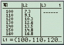
Step 2. Use the Logistic feature to find the logistic regression model.
Display values are following as,
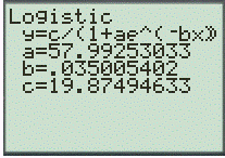
Thus, the function can be written as following,
Now, write the mode as obtained in the mentioned exercise 56 of section 3.1 of this book.
Therefore, both the modes are similar.
Chapter 3 Solutions
PRECALCULUS:...COMMON CORE ED.-W/ACCESS
- Here is a region R in Quadrant I. y 2.0 T 1.5 1.0 0.5 0.0 + 55 0.0 0.5 1.0 1.5 2.0 X It is bounded by y = x¹/3, y = 1, and x = 0. We want to evaluate this double integral. ONLY ONE order of integration will work. Good luck! The dA =???arrow_forward43–46. Directions of change Consider the following functions f and points P. Sketch the xy-plane showing P and the level curve through P. Indicate (as in Figure 15.52) the directions of maximum increase, maximum decrease, and no change for f. ■ 45. f(x, y) = x² + xy + y² + 7; P(−3, 3)arrow_forwardEX-let d'be ametric on a vector space X induced from a norm hx and d defind by a Slab)= {od (a, if a = b (a,b)+is ab Show that cannot be induced froman norm on X. 2) let à be trivel metric show that I cannot be induced from an norm on X- 3) let M be closed subspace of anormed spacex Construct the space X/Mas a normed space. 4) let Mix be vector space of 2x3 matrices on R write with Prove convex set and hyper Plane of M 5) show that every a finite dimension subspace of anormed space is closed.arrow_forward
- please do #48arrow_forward43–46. Directions of change Consider the following functions f and points P. Sketch the xy-plane showing P and the level curve through P. Indicate (as in Figure 15.52) the directions of maximum increase, maximum decrease, and no change for f. ■ 45. f(x, y) = x² + xy + y² + 7; P(−3, 3)arrow_forwardplese do #48arrow_forward
- 43-46. Directions of change Consider the following functions f and points P. Sketch the xy-plane showing P and the level curve through P. Indicate (as in Figure 15.52) the directions of maximum increase, maximum decrease, and no change for f. T 45. f(x, y) = x² + xy + y² + 7; P(−3, 3)arrow_forwardSolve the differential equation by variation of parameters 3x2y" + 7xy' + y = x2 - xarrow_forward2 x² + 9 d x 1 x +9 dxarrow_forward
 Calculus: Early TranscendentalsCalculusISBN:9781285741550Author:James StewartPublisher:Cengage Learning
 Thomas' Calculus (14th Edition)CalculusISBN:9780134438986Author:Joel R. Hass, Christopher E. Heil, Maurice D. WeirPublisher:PEARSON
 Calculus: Early Transcendentals (3rd Edition)CalculusISBN:9780134763644Author:William L. Briggs, Lyle Cochran, Bernard Gillett, Eric SchulzPublisher:PEARSON
 Calculus: Early TranscendentalsCalculusISBN:9781319050740Author:Jon Rogawski, Colin Adams, Robert FranzosaPublisher:W. H. Freeman
 Calculus: Early Transcendental FunctionsCalculusISBN:9781337552516Author:Ron Larson, Bruce H. EdwardsPublisher:Cengage Learning
