
Concept explainers
Videos
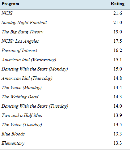
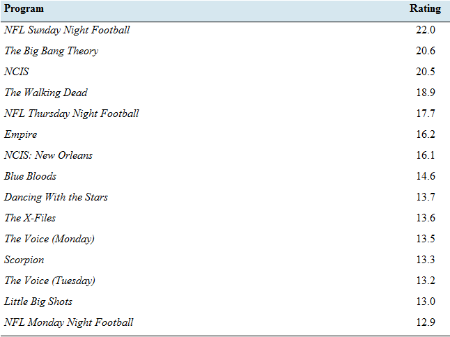
What’s your favorite TV show? The following tables present the numbers of viewers, in millions for the top 15 prime-time shows for the 2012—2013 and 2015—2016 seasons. The numbers of viewers include those who watched the program on any platform, including time-shifting up to seven days after the original telecast.

- Find the population standard deviation of the ratings for 20 12—2013.
- Find the population standard deviation of the ratings for 2015—2016.
- Compute the
range for the ratings for both seasons. - Based on the standard deviations, did the spread in ratings increase or decrease over the two seasons?
- Based on the ranges, did the spread in ratings increase or decrease over the two seasons?
a)
To find: the sample standard deviation of rating 2012 − 2013.
Answer to Problem 39E
Standard deviation = 2.74
Explanation of Solution
Given:
| Top Rated TV Programs: 2012−2013 | Top Rated TV Programs: 2015−2016 | ||
| Program | Rating | Program | Rating |
| NCIS | 21.6 | NFL Sunday Night Football | 22 |
| Sunday Night Football | 21 | The Big Bang Theory | 20.6 |
| The Big Bang Theory | 19 | NCIS | 20.5 |
| NCIS: Los Angeles | 17.5 | The Walking Dead | 18.9 |
| Person of Interest | 16.2 | NFL Thursday Night Football | 17.7 |
| American Idol (Wednesday) | 15.1 | Empire | 16.2 |
| Dancing with the Stars (Monday) | 15 | NCIS: New Orleans | 16.1 |
| American Idol (Thursday) | 14.8 | Blue Bloods | 14.6 |
| The Voice (Monday) | 14.4 | Dancing with the Stars | 13.7 |
| The Walking Dead | 14.3 | The X-Files | 13.6 |
| Dancing with the Stars (Tuesday) | 14 | The Voice (Monday) | 13.5 |
| Two and a Half Men | 13.9 | Scorpion | 13.3 |
| The Voice (Tuesday) | 13.5 | The Voice (Tuesday) | 13.2 |
| Blue Bloods | 13.3 | Little Big Shots | 13 |
| Elementary | 13.3 | NFL Monday Night Football | 12.9 |
Formula used:
Calculation:
| Top Rated TV Programs: 2012−2013 | ||
| Program | Rating | |
| NCIS | 21.6 | 33.72 |
| Sunday Night Football | 21 | 27.11 |
| The Big Bang Theory | 19 | 10.28 |
| NCIS: Los Angeles | 17.5 | 2.91 |
| Person of Interest | 16.2 | 0.17 |
| American Idol (Wednesday) | 15.1 | 0.48 |
| Dancing with the Stars (Monday) | 15 | 0.63 |
| American Idol (Thursday) | 14.8 | 0.99 |
| The Voice (Monday) | 14.4 | 1.94 |
| The Walking Dead | 14.3 | 2.23 |
| Dancing with the Stars (Tuesday) | 14 | 3.22 |
| Two and a Half Men | 13.9 | 3.58 |
| The Voice (Tuesday) | 13.5 | 5.26 |
| Blue Bloods | 13.3 | 6.22 |
| Elementary | 13.3 | 6.22 |
| Sum | 236.90 | 104.95 |
| average | 15.79 | |
| Standard deviation | 2.74 | |
b)
To find: the sample standard deviation for the rating in year 2015 − 2016.
Answer to Problem 39E
Standard deviation = 3.18
Explanation of Solution
Calculation:
| Top Rated TV Programs: 2015−2016 | ||
| Program | Rating | |
| NFL Sunday Night Football | 22 | 36.16 |
| The Big Bang Theory | 20.6 | 21.28 |
| NCIS | 20.5 | 20.37 |
| The Walking Dead | 18.9 | 8.49 |
| NFL Thursday Night Football | 17.7 | 2.94 |
| Empire | 16.2 | 0.05 |
| NCIS: New Orleans | 16.1 | 0.01 |
| Blue Bloods | 14.6 | 1.92 |
| Dancing with the Stars | 13.7 | 5.23 |
| The X-Files | 13.6 | 5.70 |
| The Voice (Monday) | 13.5 | 6.18 |
| Scorpion | 13.3 | 7.22 |
| The Voice (Tuesday) | 13.2 | 7.77 |
| Little Big Shots | 13 | 8.92 |
| NFL Monday Night Football | 12.9 | 9.53 |
| Sum | 239.8 | 141.76 |
| average | 15.99 | |
| Standard deviation | 3.18 | |
c)
To find: the range of ratings for both years.
Answer to Problem 39E
Range:
2012 − 13 = 8.3
2015 − 15 = 9.1
Explanation of Solution
Formula used:
Range = Highest Value − lowest value
Calculation:
d)
To explain: whether the spread has increase or decrease based on standard deviation of both years.
Answer to Problem 39E
Increased
Explanation of Solution
Since the standard deviation in 2012 − 2013 is 2.74 and in year 2015 − 2016 it is 3.18, which shows that the spread of rating has increased over the given time periods.
e)
To explain: whether the spread has increase or decrease based on standard deviation of both years.
Answer to Problem 39E
Increased
Explanation of Solution
Since the Range in 2012 − 2013 is 8.3 and in year 2015 − 2016 it is 9.1, which shows that the spread of rating has increased over the given time periods.
Want to see more full solutions like this?
Chapter 3 Solutions
ELEMENTARY STATISTICS-ALEKS ACCESS CODE


- (a) What is a bimodal histogram? (b) Explain the difference between left-skewed, symmetric, and right-skewed histograms. (c) What is an outlierarrow_forward(a) Test the hypothesis. Consider the hypothesis test Ho = : against H₁o < 02. Suppose that the sample sizes aren₁ = 7 and n₂ = 13 and that $² = 22.4 and $22 = 28.2. Use α = 0.05. Ho is not ✓ rejected. 9-9 IV (b) Find a 95% confidence interval on of 102. Round your answer to two decimal places (e.g. 98.76).arrow_forwardLet us suppose we have some article reported on a study of potential sources of injury to equine veterinarians conducted at a university veterinary hospital. Forces on the hand were measured for several common activities that veterinarians engage in when examining or treating horses. We will consider the forces on the hands for two tasks, lifting and using ultrasound. Assume that both sample sizes are 6, the sample mean force for lifting was 6.2 pounds with standard deviation 1.5 pounds, and the sample mean force for using ultrasound was 6.4 pounds with standard deviation 0.3 pounds. Assume that the standard deviations are known. Suppose that you wanted to detect a true difference in mean force of 0.25 pounds on the hands for these two activities. Under the null hypothesis, 40 = 0. What level of type II error would you recommend here? Round your answer to four decimal places (e.g. 98.7654). Use a = 0.05. β = i What sample size would be required? Assume the sample sizes are to be equal.…arrow_forward
- = Consider the hypothesis test Ho: μ₁ = μ₂ against H₁ μ₁ μ2. Suppose that sample sizes are n₁ = 15 and n₂ = 15, that x1 = 4.7 and X2 = 7.8 and that s² = 4 and s² = 6.26. Assume that o and that the data are drawn from normal distributions. Use απ 0.05. (a) Test the hypothesis and find the P-value. (b) What is the power of the test in part (a) for a true difference in means of 3? (c) Assuming equal sample sizes, what sample size should be used to obtain ẞ = 0.05 if the true difference in means is - 2? Assume that α = 0.05. (a) The null hypothesis is 98.7654). rejected. The P-value is 0.0008 (b) The power is 0.94 . Round your answer to four decimal places (e.g. Round your answer to two decimal places (e.g. 98.76). (c) n₁ = n2 = 1 . Round your answer to the nearest integer.arrow_forwardConsider the hypothesis test Ho: = 622 against H₁: 6 > 62. Suppose that the sample sizes are n₁ = 20 and n₂ = 8, and that = 4.5; s=2.3. Use a = 0.01. (a) Test the hypothesis. Round your answers to two decimal places (e.g. 98.76). The test statistic is fo = i The critical value is f = Conclusion: i the null hypothesis at a = 0.01. (b) Construct the confidence interval on 02/022 which can be used to test the hypothesis: (Round your answer to two decimal places (e.g. 98.76).) iarrow_forward2011 listing by carmax of the ages and prices of various corollas in a ceratin regionarrow_forward
- س 11/ أ . اذا كانت 1 + x) = 2 x 3 + 2 x 2 + x) هي متعددة حدود محسوبة باستخدام طريقة الفروقات المنتهية (finite differences) من جدول البيانات التالي للدالة (f(x . احسب قيمة . ( 2 درجة ) xi k=0 k=1 k=2 k=3 0 3 1 2 2 2 3 αarrow_forward1. Differentiate between discrete and continuous random variables, providing examples for each type. 2. Consider a discrete random variable representing the number of patients visiting a clinic each day. The probabilities for the number of visits are as follows: 0 visits: P(0) = 0.2 1 visit: P(1) = 0.3 2 visits: P(2) = 0.5 Using this information, calculate the expected value (mean) of the number of patient visits per day. Show all your workings clearly. Rubric to follow Definition of Random variables ( clearly and accurately differentiate between discrete and continuous random variables with appropriate examples for each) Identification of discrete random variable (correctly identifies "number of patient visits" as a discrete random variable and explains reasoning clearly.) Calculation of probabilities (uses the probabilities correctly in the calculation, showing all steps clearly and logically) Expected value calculation (calculate the expected value (mean)…arrow_forwardif the b coloumn of a z table disappeared what would be used to determine b column probabilitiesarrow_forward
- Construct a model of population flow between metropolitan and nonmetropolitan areas of a given country, given that their respective populations in 2015 were 263 million and 45 million. The probabilities are given by the following matrix. (from) (to) metro nonmetro 0.99 0.02 metro 0.01 0.98 nonmetro Predict the population distributions of metropolitan and nonmetropolitan areas for the years 2016 through 2020 (in millions, to four decimal places). (Let x, through x5 represent the years 2016 through 2020, respectively.) x₁ = x2 X3 261.27 46.73 11 259.59 48.41 11 257.96 50.04 11 256.39 51.61 11 tarrow_forwardIf the average price of a new one family home is $246,300 with a standard deviation of $15,000 find the minimum and maximum prices of the houses that a contractor will build to satisfy 88% of the market valuearrow_forward21. ANALYSIS OF LAST DIGITS Heights of statistics students were obtained by the author as part of an experiment conducted for class. The last digits of those heights are listed below. Construct a frequency distribution with 10 classes. Based on the distribution, do the heights appear to be reported or actually measured? Does there appear to be a gap in the frequencies and, if so, how might that gap be explained? What do you know about the accuracy of the results? 3 4 555 0 0 0 0 0 0 0 0 0 1 1 23 3 5 5 5 5 5 5 5 5 5 5 5 5 6 6 8 8 8 9arrow_forward
 Big Ideas Math A Bridge To Success Algebra 1: Stu...AlgebraISBN:9781680331141Author:HOUGHTON MIFFLIN HARCOURTPublisher:Houghton Mifflin Harcourt
 Glencoe Algebra 1, Student Edition, 9780079039897...AlgebraISBN:9780079039897Author:CarterPublisher:McGraw Hill
 Holt Mcdougal Larson Pre-algebra: Student Edition...AlgebraISBN:9780547587776Author:HOLT MCDOUGALPublisher:HOLT MCDOUGAL
 College Algebra (MindTap Course List)AlgebraISBN:9781305652231Author:R. David Gustafson, Jeff HughesPublisher:Cengage Learning