Essentials of Modern Business Statistics with Microsoft Office Excel (Book Only)

7th Edition

ISBN: 9781337681643

Author: David R. Anderson; Dennis J. Sweeney; Thomas A. Williams

Publisher: Cengage Learning US

See similar textbooks

Concept explainers

Unitary Method

The word “unitary” comes from the word “unit”, which means a single and complete entity. In this method, we find the value of a unit product from the given number of products, and then we solve for the other number of products.

Speed, Time, and Distance

Imagine you and 3 of your friends are planning to go to the playground at 6 in the evening. Your house is one mile away from the playground and one of your friends named Jim must start at 5 pm to reach the playground by walk. The other two friends are 3 …

Profit and Loss

The amount earned or lost on the sale of one or more items is referred to as the profit or loss on that item.

Units and Measurements

Measurements and comparisons are the foundation of science and engineering. We, therefore, need rules that tell us how things are measured and compared. For these measurements and comparisons, we perform certain experiments, and we will need the experime…

Videos

Textbook Question

Chapter 3, Problem 64SE

The average waiting time for a patient at an El Paso physician's office is just over 29 minutes, well above the national average of 21 minutes. In fact, El Paso has the longest physician's office waiting times in the United States (El Paso Times, January 8, 2012). In order to address the issue of long patient wait times, some physician's offices are using wait tracking systems to notify patients of expected wait times. Patients can adjust their arrival times based on this formation and spend less time in waiting rooms. 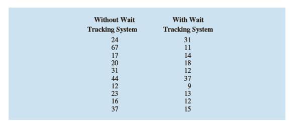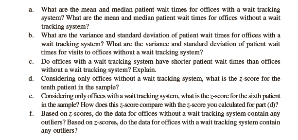The following data show wait times (minutes) for a sample of patients at offices that do not have an office tracking system and wait times for a sample of patients at offices with an office tracking system Chapter 3, Problem 64SE, The average waiting time for a patient at an El Paso physician's office is just over 29 minutes, , example 1
a.What are the mean and median patient wait times for offices with a wait tracking system? What are the mean and median patient wait times for offices without a wait tracking system?
b.What are the variance and standard deviation of patient wait times for offices with a wait tracking system? What are the variance and standard deviation of patient wait times for visits to offices without a wait tracking system?
c.Do offices with a wait tracking system have shorter patient wait times than offices without a wait tracking system? Explain.
d.Considering only offices without a wait tracking system, what is the z-score for the tenth patient in the sample?
e.Considering only offices with a wait tracking system, what is the z-score for the sixth patient in the sample? How does this z-score compare with the z-score you calculated for pat (d)?
f.Based on z-scores, do the data for offices without a wait tracking system contain any outliers? Based on z-scores, do the data for offices with a wait tracking system contain any outliers?

Chapter 3, Problem 64SE, The average waiting time for a patient at an El Paso physician's office is just over 29 minutes, , example 2

Definition Definition Measure of central tendency that is the average of a given data set. The mean value is evaluated as the quotient of the sum of all observations by the sample size. The mean, in contrast to a median, is affected by extreme values. Very large or very small values can distract the mean from the center of the data. Arithmetic mean: The most common type of mean is the arithmetic mean. It is evaluated using the formula: μ = 1 N ∑ i = 1 N x i Other types of means are the geometric mean, logarithmic mean, and harmonic mean. Geometric mean: The nth root of the product of n observations from a data set is defined as the geometric mean of the set: G = x 1 x 2 ... x n n Logarithmic mean: The difference of the natural logarithms of the two numbers, divided by the difference between the numbers is the logarithmic mean of the two numbers. The logarithmic mean is used particularly in heat transfer and mass transfer. ln x 2 − ln x 1 x 2 − x 1 Harmonic mean: The inverse of the arithmetic mean of the inverses of all the numbers in a data set is the harmonic mean of the data. 1 1 x 1 + 1 x 2 + ...

Expert Solution & Answer

Want to see the full answer?

Check out a sample textbook solution

See solution

Chapter 3, Problem 63SE

Chapter 3, Problem 65SE

Students have asked these similar questions

08:34 ◄ Classroom 07:59 Probs. 5-32/33 D ا. 89 5-34. Determine the horizontal and vertical components of reaction at the pin A and the normal force at the smooth peg B on the member. A 0,4 m 0.4 m Prob. 5-34 F=600 N fr th ar 0. 163586 5-37. The wooden plank resting between the buildings deflects slightly when it supports the 50-kg boy. This deflection causes a triangular distribution of load at its ends. having maximum intensities of w, and wg. Determine w and wg. each measured in N/m. when the boy is standing 3 m from one end as shown. Neglect the mass of the plank. 0.45 m 3 m

Examine the Variables: Carefully review and note the names of all variables in the dataset. Examples of these variables include: Mileage (mpg) Number of Cylinders (cyl) Displacement (disp) Horsepower (hp) Research: Google to understand these variables. Statistical Analysis: Select mpg variable, and perform the following statistical tests. Once you are done with these tests using mpg variable, repeat the same with hp Mean Median First Quartile (Q1) Second Quartile (Q2) Third Quartile (Q3) Fourth Quartile (Q4) 10th Percentile 70th Percentile Skewness Kurtosis Document Your Results: In RStudio: Before running each statistical test, provide a heading in the format shown at the bottom. “# Mean of mileage – Your name’s command” In Microsoft Word: Once you've completed all tests, take a screenshot of your results in RStudio and paste it into a Microsoft Word document. Make sure that snapshots are very clear. You will need multiple snapshots. Also transfer these results to the…

Chapter 3 Solutions

Essentials of Modern Business Statistics with Microsoft Office Excel (Book Only)

Ch. 3.1 - Consider a sample with data values of 10, 20, 12,...Ch. 3.1 - Consider a sample with data values of 10, 20, 21,...Ch. 3.1 - Consider the following data and corresponding...Ch. 3.1 - Consider the following data. What is the mean...Ch. 3.1 - Prob. 5E Ch. 3.1 - Prob. 6E Ch. 3.1 - The average number of minutes Americans commute to...Ch. 3.1 - The WWI Street Journal reported that the median...Ch. 3.1 - Which companies spend the most money on...Ch. 3.1 - Prob. 10E

Knowledge Booster

$Statistics$

Learn more about

Need a deep-dive on the concept behind this application? Look no further. Learn more about this topic, statistics and related others by exploring similar questions and additional content below.

Solution Summary: The author calculates the mean and median patient wait times for offices with and without wait tracking system.

Concept explainers

Videos

Want to see the full answer?

Chapter 3 Solutions