When mathematicians are presented with a linear programming problem, they will not only determine the optimal solution but will also supply what are called shadow prices for each resource. This chapter project develops the concept of a shadow price.
Consider the furniture manufacturing problem. The constraint for finishing is
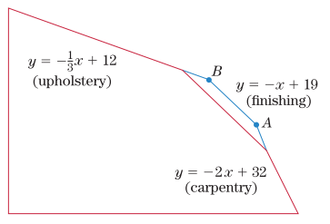
Determine the optimal solution for the revised linear programming problem. What is the new maximum profit? By how much was the profit increased due to the additional hour for finishing? This amount is the shadow price.
Want to see the full answer?
Check out a sample textbook solutionChapter 3 Solutions
EBK FINITE MATHEMATICS & ITS APPLICATIO
- Refer to page 9 for a problem requiring finding the tangent plane to a given surface at a point. Instructions: Use partial derivatives to calculate the equation of the tangent plane. Show all calculations step-by-step. Link [https://drive.google.com/file/d/1wKSrun-GlxirS31Z9qoHazb9tC440AZF/view?usp=sharing]arrow_forwardRefer to page 8 for a problem involving solving a second-order linear homogeneous differential equation. Instructions: Solve using characteristic equations. Show all intermediate steps leading to the general solution. Link: [https://drive.google.com/file/d/1wKSrun-GlxirS3IZ9qoHazb9tC440AZF/view?usp=sharing]arrow_forwardRefer to page 17 for a problem requiring solving a nonlinear algebraic equation using the bisection method. Instructions: Show iterative calculations for each step, ensuring convergence criteria are satisfied. Clearly outline all steps. Link [https://drive.google.com/file/d/1wKSrun-GlxirS31Z9qo Hazb9tC440AZF/view?usp=sharing]arrow_forward
- Problem: The probability density function of a random variable is given by the exponential distribution Find the probability that f(x) = {0.55e−0.55x 0 < x, O elsewhere} a. the time to observe a particle is more than 200 microseconds. b. the time to observe a particle is less than 10 microseconds.arrow_forwardThe OU process studied in the previous problem is a common model for interest rates. Another common model is the CIR model, which solves the SDE: dX₁ = (a = X₁) dt + σ √X+dWt, - under the condition Xoxo. We cannot solve this SDE explicitly. = (a) Use the Brownian trajectory simulated in part (a) of Problem 1, and the Euler scheme to simulate a trajectory of the CIR process. On a graph, represent both the trajectory of the OU process and the trajectory of the CIR process for the same Brownian path. (b) Repeat the simulation of the CIR process above M times (M large), for a large value of T, and use the result to estimate the long-term expectation and variance of the CIR process. How do they compare to the ones of the OU process? Numerical application: T = 10, N = 500, a = 0.04, x0 = 0.05, σ = 0.01, M = 1000. 1 (c) If you use larger values than above for the parameters, such as the ones in Problem 1, you may encounter errors when implementing the Euler scheme for CIR. Explain why.arrow_forwardRefer to page 1 for a problem involving proving the distributive property of matrix multiplication. Instructions: Provide a detailed proof using matrix definitions and element-wise operations. Show all calculations clearly. Link [https://drive.google.com/file/d/1wKSrun-GlxirS3IZ9qoHazb9tC440AZF/view?usp=sharing]arrow_forward
- Refer to page 30 for a problem requiring solving a nonhomogeneous differential equation using the method of undetermined coefficients. Instructions: Solve step-by-step, including the complementary and particular solutions. Clearly justify each step. Link [https://drive.google.com/file/d/1wKSrun-GlxirS3IZ9qoHazb9tC440AZF/view?usp=sharing]arrow_forwardRefer to page 5 for a problem requiring finding the critical points of a multivariable function. Instructions: Use partial derivatives and the second partial derivative test to classify the critical points. Provide detailed calculations. Link [https://drive.google.com/file/d/1wKSrun-GlxirS31Z9qo Hazb9tC440AZF/view?usp=sharing]arrow_forwardRefer to page 3 for a problem on evaluating limits involving indeterminate forms using L'Hôpital's rule. Instructions: Apply L'Hôpital's rule rigorously. Show all derivatives and justify the steps leading to the solution. Link [https://drive.google.com/file/d/1wKSrun-GlxirS31Z9qo Hazb9tC440AZF/view?usp=sharing]arrow_forward
- 3. Let {X} be an autoregressive process of order one, usually written as AR(1). (a) Write down an equation defining X₁ in terms of an autoregression coefficient a and a white noise process {} with variance σ². Explain what the phrase "{} is a white noise process with variance o?" means. (b) Derive expressions for the variance 70 and the autocorrelation function Pk, k 0,1,. of the {X} in terms of o2 and a. Use these expressions to suggest an estimate of a in terms of the sample autocor- relations {k}. (c) Suppose that only every second value of X is observed, resulting in a time series Y X2, t = 1, 2,.... Show that {Y} forms an AR(1) process. Find its autoregression coefficient, say d', and the variance of the underlying white noise process, in terms of a and o². (d) Given a time series data set X1, ..., X256 with sample mean = 9.23 and sample autocorrelations ₁ = -0.6, 2 = 0.36, 3 = -0.22, p = 0.13, 5 = -0.08, estimate the autoregression coefficients a and a' of {X} and {Y}.arrow_forward#8 (a) Find the equation of the tangent line to y = √x+3 at x=6 (b) Find the differential dy at y = √x +3 and evaluate it for x=6 and dx = 0.3arrow_forwardRefer to page 96 for a problem involving the heat equation. Solve the PDE using the method of separation of variables. Derive the solution step-by-step, including the boundary conditions. Instructions: Stick to solving the heat equation. Show all intermediate steps, including separation of variables, solving for eigenvalues, and constructing the solution. Irrelevant explanations are not allowed. Link: [https://drive.google.com/file/d/1wKSrun-GlxirS31Z9qoHazb9tC440AZF/view?usp=sharing]arrow_forward
- Algebra for College StudentsAlgebraISBN:9781285195780Author:Jerome E. Kaufmann, Karen L. SchwittersPublisher:Cengage LearningCollege Algebra (MindTap Course List)AlgebraISBN:9781305652231Author:R. David Gustafson, Jeff HughesPublisher:Cengage LearningElementary Geometry For College Students, 7eGeometryISBN:9781337614085Author:Alexander, Daniel C.; Koeberlein, Geralyn M.Publisher:Cengage,
- Glencoe Algebra 1, Student Edition, 9780079039897...AlgebraISBN:9780079039897Author:CarterPublisher:McGraw HillElementary Linear Algebra (MindTap Course List)AlgebraISBN:9781305658004Author:Ron LarsonPublisher:Cengage Learning