
Concept explainers
Videos
a.
To explain: The area within 1 standard deviation of the
To compare: The area within 1 standard deviation of the mean by using applet and
a.
Answer to Problem 3.52E
The area within 1 standard deviation of the mean is 0.6826.
The area within 1 standard deviation of the mean by using applet and 68-95-99.7 rule is both approximately equal.
Explanation of Solution
Given info:
The mean and standard deviation of the
68-95-99.7 Rule:
About 68% of the observations fall within
About 95% of the observations fall within
About 99.7% of the observations fall within
Calculation:
Find the area of 1 standard deviation on either side of the mean using the normal density curve applet.
Applet procedure:
Step-by-step Applet procedure to find the area of 1 standard deviation on either side of the mean is given as follows:
- In Statistical Applets, choose Normal Density Curve.
- In the normal density curve drag one flag and place at 1 standard deviation on either side of the mean.
Output obtained from Applet:
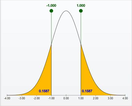
From the Applet output, the area of one standard deviation below −1 is 0.1587 and the above 1 is 0.1587.
The formula to find the area within 1 standard deviation of the mean is,
Thus, the area within 1 standard deviation of the mean is 0.6826. That is, about 68% of the observations fall within
From the 68-95-99.7 rule, the area within 1 standard deviation of the mean is about 68%.
Justification:
The result of the area within 1 standard deviation of the mean is approximately same by using the applet and the 68-95-99.7 rule.
b.
To explain: The area within 2 standard deviations of the mean and the area within 3 standard deviations of the mean.
To compare: The area within 2 standard deviations of the mean and the area within 3 standard deviations of the mean by using applet and 68-95-99.7 rule.
b.
Answer to Problem 3.52E
The area within 2 standard deviations of the mean is 0.9544 and the area within 3 standard deviations of the mean is 0.9974.
The area within 2 standard deviations of the mean by using applet and 68-95-99.7 rule is both approximately equal and the area within 3 standard deviations of the mean by using applet and 68-95-99.7 rule is both approximately equal.
Explanation of Solution
Calculation:
Finding the area of 2 standard deviations on either side of the mean:
Applet procedure:
Step-by-step Applet procedure to find the area of 2 standard deviations on either side of the mean is given as follows
- In Statistical Applets, choose Normal Density Curve.
- In the normal density curve drag one flag and place at 2 standard deviations on either side of the mean.
Output obtained from Applet:
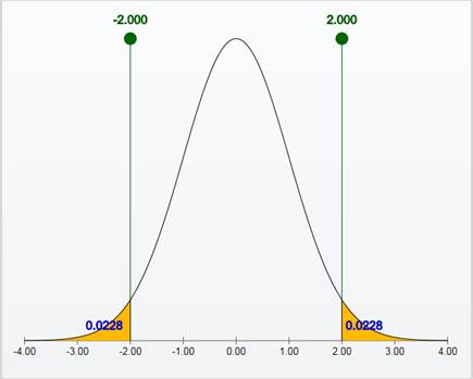
From the Applet output, the area to the left of −2 is 0.0228 and the area to right of 2 is 0.0228.
The formula to find the area within 2 standard deviations of the mean is,
Thus, the area within 2 standard deviations of the mean is 0.9544. That is, about 95% of the observations fall within
From the 68-95-99.7 rule, the area within 2 standard deviations of the mean is about 95%.
Finding the area of 3 standard deviations on either side of the mean:
Applet Procedure:
Step-by-step Applet procedure to find the area of 3 standard deviations on either side of the mean is given as follows
- In Statistical Applets, choose Normal Density Curve.
- In the normal density curve drag one flag and place at 3 standard deviations on either side of the mean.
Output obtained from Applet:
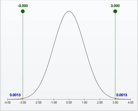
From the Applet output, the area to the left of −3 is 0.0013 and the area to right of 3 is 0.0013.
The formula to find the area within 3 standard deviations of the mean is,
Thus, the area within 3 standard deviations of the mean is 0.9974. That is, about 99.7% of the observations fall within
From the 68-95-99.7 rule, the area within 3 standard deviations of the mean is about 99.7%.
Justification:
The result of the area within 2 standard deviations of the mean is approximately same by using the applet and the 68-95-99.7 rule and also the result of the area within 3 standard deviations of the mean is approximately same by using the applet and the 68-95-99.7 rule.
Want to see more full solutions like this?
Chapter 3 Solutions
Loose-leaf Version for The Basic Practice of Statistics 7e & LaunchPad (Twelve Month Access)


- Binomial Prob. Question: A new teaching method claims to improve student engagement. A survey reveals that 60% of students find this method engaging. If 15 students are randomly selected, what is the probability that: a) Exactly 9 students find the method engaging?b) At least 7 students find the method engaging? (2 points = 1 x 2 answers) Provide answers in the yellow cellsarrow_forwardIn a survey of 2273 adults, 739 say they believe in UFOS. Construct a 95% confidence interval for the population proportion of adults who believe in UFOs. A 95% confidence interval for the population proportion is ( ☐, ☐ ). (Round to three decimal places as needed.)arrow_forwardFind the minimum sample size n needed to estimate μ for the given values of c, σ, and E. C=0.98, σ 6.7, and E = 2 Assume that a preliminary sample has at least 30 members. n = (Round up to the nearest whole number.)arrow_forward
- In a survey of 2193 adults in a recent year, 1233 say they have made a New Year's resolution. Construct 90% and 95% confidence intervals for the population proportion. Interpret the results and compare the widths of the confidence intervals. The 90% confidence interval for the population proportion p is (Round to three decimal places as needed.) J.D) .arrow_forwardLet p be the population proportion for the following condition. Find the point estimates for p and q. In a survey of 1143 adults from country A, 317 said that they were not confident that the food they eat in country A is safe. The point estimate for p, p, is (Round to three decimal places as needed.) ...arrow_forward(c) Because logistic regression predicts probabilities of outcomes, observations used to build a logistic regression model need not be independent. A. false: all observations must be independent B. true C. false: only observations with the same outcome need to be independent I ANSWERED: A. false: all observations must be independent. (This was marked wrong but I have no idea why. Isn't this a basic assumption of logistic regression)arrow_forward
- Business discussarrow_forwardSpam filters are built on principles similar to those used in logistic regression. We fit a probability that each message is spam or not spam. We have several variables for each email. Here are a few: to_multiple=1 if there are multiple recipients, winner=1 if the word 'winner' appears in the subject line, format=1 if the email is poorly formatted, re_subj=1 if "re" appears in the subject line. A logistic model was fit to a dataset with the following output: Estimate SE Z Pr(>|Z|) (Intercept) -0.8161 0.086 -9.4895 0 to_multiple -2.5651 0.3052 -8.4047 0 winner 1.5801 0.3156 5.0067 0 format -0.1528 0.1136 -1.3451 0.1786 re_subj -2.8401 0.363 -7.824 0 (a) Write down the model using the coefficients from the model fit.log_odds(spam) = -0.8161 + -2.5651 + to_multiple + 1.5801 winner + -0.1528 format + -2.8401 re_subj(b) Suppose we have an observation where to_multiple=0, winner=1, format=0, and re_subj=0. What is the predicted probability that this message is spam?…arrow_forwardConsider an event X comprised of three outcomes whose probabilities are 9/18, 1/18,and 6/18. Compute the probability of the complement of the event. Question content area bottom Part 1 A.1/2 B.2/18 C.16/18 D.16/3arrow_forward
- John and Mike were offered mints. What is the probability that at least John or Mike would respond favorably? (Hint: Use the classical definition.) Question content area bottom Part 1 A.1/2 B.3/4 C.1/8 D.3/8arrow_forwardThe details of the clock sales at a supermarket for the past 6 weeks are shown in the table below. The time series appears to be relatively stable, without trend, seasonal, or cyclical effects. The simple moving average value of k is set at 2. What is the simple moving average root mean square error? Round to two decimal places. Week Units sold 1 88 2 44 3 54 4 65 5 72 6 85 Question content area bottom Part 1 A. 207.13 B. 20.12 C. 14.39 D. 0.21arrow_forwardThe details of the clock sales at a supermarket for the past 6 weeks are shown in the table below. The time series appears to be relatively stable, without trend, seasonal, or cyclical effects. The simple moving average value of k is set at 2. If the smoothing constant is assumed to be 0.7, and setting F1 and F2=A1, what is the exponential smoothing sales forecast for week 7? Round to the nearest whole number. Week Units sold 1 88 2 44 3 54 4 65 5 72 6 85 Question content area bottom Part 1 A. 80 clocks B. 60 clocks C. 70 clocks D. 50 clocksarrow_forward
 MATLAB: An Introduction with ApplicationsStatisticsISBN:9781119256830Author:Amos GilatPublisher:John Wiley & Sons Inc
 Probability and Statistics for Engineering and th...StatisticsISBN:9781305251809Author:Jay L. DevorePublisher:Cengage Learning
 Statistics for The Behavioral Sciences (MindTap C...StatisticsISBN:9781305504912Author:Frederick J Gravetter, Larry B. WallnauPublisher:Cengage Learning
 Elementary Statistics: Picturing the World (7th E...StatisticsISBN:9780134683416Author:Ron Larson, Betsy FarberPublisher:PEARSON
 The Basic Practice of StatisticsStatisticsISBN:9781319042578Author:David S. Moore, William I. Notz, Michael A. FlignerPublisher:W. H. Freeman
 Introduction to the Practice of StatisticsStatisticsISBN:9781319013387Author:David S. Moore, George P. McCabe, Bruce A. CraigPublisher:W. H. Freeman