
a.
To draw: A histogram with a superimposed normal curve.
a.
Answer to Problem 3.49E
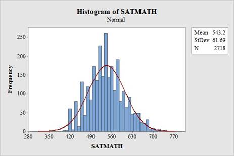
The obtained histogram with a superimposed normal curve is,
Explanation of Solution
Given info:
The data of SATMATH are given.
Calculation:
Histogram:
Software Procedure:
Step by step procedure to obtain Histogram is given as:
- Choose Graph > Histogram.
- Choose With Fit, and then click OK.
- In Graph variables, enter the corresponding data column SATMATH.
- Click OK.
The output using Minitab software is given as:
b.
To find: The
To compare: The mean and the median.
To compare: The quartiles.
b.
Answer to Problem 3.49E
The mean, median, standard deviation, 1st quartile, 2nd quartile are 543.2, 540, 61.69, 500 and 580, respectively.
The distribution is symmetric.
Explanation of Solution
Calculation:
Software Procedure:
Step by step procedure to obtain the inter
- Choose Stat > Basic Statistics > Display Descriptive Statistics.
- In Variables enter the columns SAT.
- In statistics choose Mean, Median, Standard deviation, 1st quartile, 3rd quartile..
- Click OK.
Output using the MINITAB software is given below:
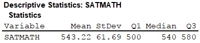
From the MINITAB output,
The mean is 543.2.
The standard deviation is 61.69.
The 1st quartile is 500.
The median is 540.
The 3rd quartile is 580.
Comparison between mean and median:
If mean is equal to the median then it is said to be symmetric.
Here, the mean is close to the median. Thus, the distribution is symmetric.
Distance of the first quartile from the median:
The formula to find the distance of the first quartile from the median is,
Thus, the distance of the first quartile from the median is 40.
Distance of the first quartile from the median:
The formula to find the distance of the third quartile from the median is,
Thus, the distance of the third quartile from the median is 40.
Here, the distance of the first quartile from the median is approximately equal to distance of the third quartile from the median. That is,
Hence, the distribution of the rainwater specimens is quite symmetric.
c.
To find: The proportion of GSU freshmen scored above the mean 514 for all college-bound seniors.
c.
Answer to Problem 3.49E
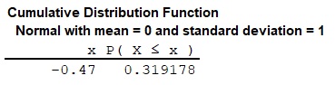
The proportion of GSU freshmen scored above the mean 514 for all college-bound seniors is 0.6808.
Explanation of Solution
The formula to find the standardized score is,
In 2013, the mean score on the mathematics portion of the SAT for all college-bound seniors was 514.
The distribution of first 20 SAT mathematics scores follow
Consider the random variable X, denotes those students of first 20 SAT mathematics scores.
Thus,
It is known that,
Thus,
Cumulative probability value:
Software Procedure:
Step by step procedure to obtain the graph using the MINITAB software:
- Choose Calc > Probability distribution> Normal.
- Choose Cumulative Probability.
- In mean, enter 0.
- In standard deviation, enter 1.
- Choose Input Constant.
- In Input Constant, enter -0.47.
- Click OK.
Output using the MINITAB software is given below:
Thus,
Therefore, the proportion of GSU freshmen scored above the mean for all college-bound seniors is 0.6808.
d.
To find: The exact proportion of GSU freshmen who scored above the mean for all college-bound seniors.
d.
Answer to Problem 3.49E
The exact proportion of GSU freshmen who scored above the mean for all college-bound seniors is 0.6840.
Explanation of Solution
It is found from the data that 1,859 students, out of a total of 2,718 students have scored above the mean score 514 for all college-bound seniors.
Thus, the exact proportion of GSU freshmen who scored above the mean for all college-bound seniors is:
From part (c), the proportion of GSU freshmen scored above the mean 514 for all college-bound seniors, for normal distribution is 0.6808 or 68.08%.
Here, the exact proportion of GSU freshmen who scored above the mean for all college-bound seniors is 0.6840 or 68.40%.
It can be said that
Thus, the exact percentage obtained from part (d) and the percentage obtained from part (c) are very close.
Thus, despite any discrepancies, the distribution can be considered to be “close enough to Normal” distribution.
Want to see more full solutions like this?
Chapter 3 Solutions
The Basic Practice of Statistics

- The scores of 8 students on the midterm exam and final exam were as follows. Student Midterm Final Anderson 98 89 Bailey 88 74 Cruz 87 97 DeSana 85 79 Erickson 85 94 Francis 83 71 Gray 74 98 Harris 70 91 Find the value of the (Spearman's) rank correlation coefficient test statistic that would be used to test the claim of no correlation between midterm score and final exam score. Round your answer to 3 places after the decimal point, if necessary. Test statistic: rs =arrow_forwardBusiness discussarrow_forwardBusiness discussarrow_forward
- I just need to know why this is wrong below: What is the test statistic W? W=5 (incorrect) and What is the p-value of this test? (p-value < 0.001-- incorrect) Use the Wilcoxon signed rank test to test the hypothesis that the median number of pages in the statistics books in the library from which the sample was taken is 400. A sample of 12 statistics books have the following numbers of pages pages 127 217 486 132 397 297 396 327 292 256 358 272 What is the sum of the negative ranks (W-)? 75 What is the sum of the positive ranks (W+)? 5What type of test is this? two tailedWhat is the test statistic W? 5 These are the critical values for a 1-tailed Wilcoxon Signed Rank test for n=12 Alpha Level 0.001 0.005 0.01 0.025 0.05 0.1 0.2 Critical Value 75 70 68 64 60 56 50 What is the p-value for this test? p-value < 0.001arrow_forwardons 12. A sociologist hypothesizes that the crime rate is higher in areas with higher poverty rate and lower median income. She col- lects data on the crime rate (crimes per 100,000 residents), the poverty rate (in %), and the median income (in $1,000s) from 41 New England cities. A portion of the regression results is shown in the following table. Standard Coefficients error t stat p-value Intercept -301.62 549.71 -0.55 0.5864 Poverty 53.16 14.22 3.74 0.0006 Income 4.95 8.26 0.60 0.5526 a. b. Are the signs as expected on the slope coefficients? Predict the crime rate in an area with a poverty rate of 20% and a median income of $50,000. 3. Using data from 50 workarrow_forward2. The owner of several used-car dealerships believes that the selling price of a used car can best be predicted using the car's age. He uses data on the recent selling price (in $) and age of 20 used sedans to estimate Price = Po + B₁Age + ε. A portion of the regression results is shown in the accompanying table. Standard Coefficients Intercept 21187.94 Error 733.42 t Stat p-value 28.89 1.56E-16 Age -1208.25 128.95 -9.37 2.41E-08 a. What is the estimate for B₁? Interpret this value. b. What is the sample regression equation? C. Predict the selling price of a 5-year-old sedan.arrow_forward
- ian income of $50,000. erty rate of 13. Using data from 50 workers, a researcher estimates Wage = Bo+B,Education + B₂Experience + B3Age+e, where Wage is the hourly wage rate and Education, Experience, and Age are the years of higher education, the years of experience, and the age of the worker, respectively. A portion of the regression results is shown in the following table. ni ogolloo bash 1 Standard Coefficients error t stat p-value Intercept 7.87 4.09 1.93 0.0603 Education 1.44 0.34 4.24 0.0001 Experience 0.45 0.14 3.16 0.0028 Age -0.01 0.08 -0.14 0.8920 a. Interpret the estimated coefficients for Education and Experience. b. Predict the hourly wage rate for a 30-year-old worker with four years of higher education and three years of experience.arrow_forward1. If a firm spends more on advertising, is it likely to increase sales? Data on annual sales (in $100,000s) and advertising expenditures (in $10,000s) were collected for 20 firms in order to estimate the model Sales = Po + B₁Advertising + ε. A portion of the regression results is shown in the accompanying table. Intercept Advertising Standard Coefficients Error t Stat p-value -7.42 1.46 -5.09 7.66E-05 0.42 0.05 8.70 7.26E-08 a. Interpret the estimated slope coefficient. b. What is the sample regression equation? C. Predict the sales for a firm that spends $500,000 annually on advertising.arrow_forwardCan you help me solve problem 38 with steps im stuck.arrow_forward
- How do the samples hold up to the efficiency test? What percentages of the samples pass or fail the test? What would be the likelihood of having the following specific number of efficiency test failures in the next 300 processors tested? 1 failures, 5 failures, 10 failures and 20 failures.arrow_forwardThe battery temperatures are a major concern for us. Can you analyze and describe the sample data? What are the average and median temperatures? How much variability is there in the temperatures? Is there anything that stands out? Our engineers’ assumption is that the temperature data is normally distributed. If that is the case, what would be the likelihood that the Safety Zone temperature will exceed 5.15 degrees? What is the probability that the Safety Zone temperature will be less than 4.65 degrees? What is the actual percentage of samples that exceed 5.25 degrees or are less than 4.75 degrees? Is the manufacturing process producing units with stable Safety Zone temperatures? Can you check if there are any apparent changes in the temperature pattern? Are there any outliers? A closer look at the Z-scores should help you in this regard.arrow_forwardNeed help pleasearrow_forward
 MATLAB: An Introduction with ApplicationsStatisticsISBN:9781119256830Author:Amos GilatPublisher:John Wiley & Sons Inc
 Probability and Statistics for Engineering and th...StatisticsISBN:9781305251809Author:Jay L. DevorePublisher:Cengage Learning
 Statistics for The Behavioral Sciences (MindTap C...StatisticsISBN:9781305504912Author:Frederick J Gravetter, Larry B. WallnauPublisher:Cengage Learning
 Elementary Statistics: Picturing the World (7th E...StatisticsISBN:9780134683416Author:Ron Larson, Betsy FarberPublisher:PEARSON
 The Basic Practice of StatisticsStatisticsISBN:9781319042578Author:David S. Moore, William I. Notz, Michael A. FlignerPublisher:W. H. Freeman
 Introduction to the Practice of StatisticsStatisticsISBN:9781319013387Author:David S. Moore, George P. McCabe, Bruce A. CraigPublisher:W. H. Freeman