Chapter 3, Problem 3.28E

a.

To determine

To explain: The type of graph could be used to explain the relationship between the two variables.

Explanation of Solution

Given:

The data set is:

Temperature	Percent
13.34	4.39
13.59	4.39
13.66	5.63
13.83	6.3
13.95	5.49
14.01	4.1
14.13	4.1
14.19	5.29
14.24	5.1
14.24	4.41
14.28	5.01
14.37	5.8
14.45	4.75
14.47	5.48
14.53	6.09
14.53	5.59
14.62	4.82
14.69	5.12
14.71	5.23
14.76	4.39
14.82	5.81
14.9	5.5
14.91	5.84
14.92	4.36
15.02	4.91
15.06	4.99
15.09	3.7
15.19	6.21
15.21	6.21
15.22	4.1
15.33	4.1
15.36	4.69
15.4	5.6
15.44	3.51
15.53	5.91
15.56	3.99
15.61	3.59
15.65	4.18
15.8	3.8
15.91	3.61
15.98	3.3
16.02	3.8
16.06	3.49
16.13	3.19
16.14	6
16.22	3.5
16.34	2.8
16.42	3.61
16.71	2
16.74	3.5
16.84	3
17.17	3.61
17.51	2.97

The scatter plot is a visual representation of two continuous type variables which shows the relationship between two variables. It tells the level of correlation between two variables. The one of the two variables can be called as explanatory variables and the other as response variable. Thus, in this case scatter plot could be used to find the association between the two variables.

b.

To determine

To compare: The analysis for the 2D system with that of 3D system and explain whether 3D program is an improved version over the 2D version.

Explanation of Solution

In this case, temperature is an explanatory variables as it does not get affected by any other variables

Graph:

The scatter plot for the provided variables can be constructed as:

  

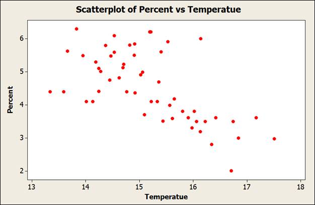
From the scatter plot constructed above,

Direction: There is a negative association between the two variables

Form: There is approximately linear relationship between the variables.

Strength: There is a moderate negative relationship between variables

c.

To determine

To find: The numerical value of the correlation, if possible and explain the association using the value of the correlation coefficient.

Explanation of Solution

The correlation using the mentioned steps of Excel below can be calculated as:

1. Enter the data set in the Excel sheet.
2. Click on Data > Data Analysis.
3. Select “Correlation” from the drop down menu.
4. Select input range.
5. Click OK.

The obtained output is:

  

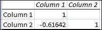
Thus, the correlation coefficient ( r ) is approximately -0.62. Thus, it is confirmed that there is a moderate negative correlation between the two variables. It implies that increase in increase in temperature tends to decrease the $\alpha -$ content in hops and vice versa