
Concept explainers
Videos
a
Identify the sampling plan that can be preferred, if the seller produces lots with fraction defective
a
Answer to Problem 183SE
The sampling plan that can be preferred, if the seller produces lots with fraction defective ranging from
Explanation of Solution
Calculation:
Binomial distribution:
A random variable Y is a binomial distribution based on n trails with success
For sampling plan 1 with
The probability of acceptance for
The probability of acceptance for
The probability of acceptance for
The probability of acceptance for
The probability of acceptance for
The probability of acceptance for sampling plan
| p | 0.05 | 0.10 | 0.20 | 0.30 | 0.40 |
| 0.9774 | 0.9186 | 0.7373 | 0.5283 | 0.3370 |
For sampling plan 2 with
The probability of acceptance for
The probability of acceptance for
The probability of acceptance for
The probability of acceptance for
The probability of acceptance for
The probability of acceptance for sampling plan
| p | 0.05 | 0.10 | 0.20 | 0.30 | 0.40 |
| 0.9987 | 0.9666 | 0.6165 | 0.1934 | 0.02936 |
Step by step procedure to construct OC curve:
- In OC curve, take the values of probability p on x-axis.
- Take the values of probability of acceptance for p on y-axis.
- Locate the value of probability of acceptance 0.0059 corresponding to probability 0.05 for sampling plan 1.
- Similarly locate all the probability values for both the sampling plans.
- Connect all the dots with a curved line to form the OC curve.
The OC curve is,
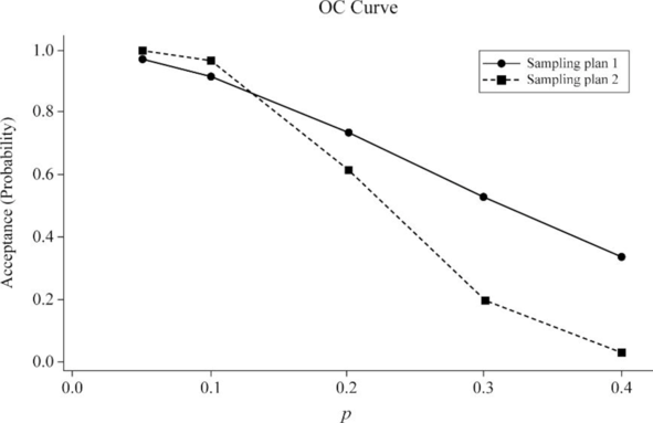
From the OC curve it can be observed that, for the interval
Hence, the sampling plan that can be preferred, if the seller produces lots with fraction defective ranging from
b
Identify the sampling plan that can be preferred, if the seller produces lots with fraction defective exceeding
b
Answer to Problem 183SE
The sampling plan that can be preferred, if the seller produces lots with fraction defective exceeding
Explanation of Solution
From the OC curve of part (a), it can be observed that, for the p values exceeding 0.30, the line for sampling plan 2 is above the line of sampling plan 1. This shows that, using sampling plan 2 would be preferable if the seller produces lots with fraction defective exceeding 0.30.
Hence, the sampling plan that can be preferred, if the seller produces lots with fraction defective exceeding
Want to see more full solutions like this?
Chapter 3 Solutions
Mathematical Statistics with Applications


- Please help me with the following question on statisticsFor question (e), the drop down options are: (From this data/The census/From this population of data), one can infer that the mean/average octane rating is (less than/equal to/greater than) __. (use one decimal in your answer).arrow_forwardHelp me on the following question on statisticsarrow_forward3. [15] The joint PDF of RVS X and Y is given by fx.x(x,y) = { x) = { c(x + { c(x+y³), 0, 0≤x≤ 1,0≤ y ≤1 otherwise where c is a constant. (a) Find the value of c. (b) Find P(0 ≤ X ≤,arrow_forwardNeed help pleasearrow_forward7. [10] Suppose that Xi, i = 1,..., 5, are independent normal random variables, where X1, X2 and X3 have the same distribution N(1, 2) and X4 and X5 have the same distribution N(-1, 1). Let (a) Find V(X5 - X3). 1 = √(x1 + x2) — — (Xx3 + x4 + X5). (b) Find the distribution of Y. (c) Find Cov(X2 - X1, Y). -arrow_forward1. [10] Suppose that X ~N(-2, 4). Let Y = 3X-1. (a) Find the distribution of Y. Show your work. (b) Find P(-8< Y < 15) by using the CDF, (2), of the standard normal distribu- tion. (c) Find the 0.05th right-tail percentage point (i.e., the 0.95th quantile) of the distri- bution of Y.arrow_forward6. [10] Let X, Y and Z be random variables. Suppose that E(X) = E(Y) = 1, E(Z) = 2, V(X) = 1, V(Y) = V(Z) = 4, Cov(X,Y) = -1, Cov(X, Z) = 0.5, and Cov(Y, Z) = -2. 2 (a) Find V(XY+2Z). (b) Find Cov(-x+2Y+Z, -Y-2Z).arrow_forward1. [10] Suppose that X ~N(-2, 4). Let Y = 3X-1. (a) Find the distribution of Y. Show your work. (b) Find P(-8< Y < 15) by using the CDF, (2), of the standard normal distribu- tion. (c) Find the 0.05th right-tail percentage point (i.e., the 0.95th quantile) of the distri- bution of Y.arrow_forward== 4. [10] Let X be a RV. Suppose that E[X(X-1)] = 3 and E(X) = 2. (a) Find E[(4-2X)²]. (b) Find V(-3x+1).arrow_forward2. [15] Let X and Y be two discrete RVs whose joint PMF is given by the following table: y Px,y(x, y) -1 1 3 0 0.1 0.04 0.02 I 2 0.08 0.2 0.06 4 0.06 0.14 0.30 (a) Find P(X ≥ 2, Y < 1). (b) Find P(X ≤Y - 1). (c) Find the marginal PMFs of X and Y. (d) Are X and Y independent? Explain (e) Find E(XY) and Cov(X, Y).arrow_forward32. Consider a normally distributed population with mean μ = 80 and standard deviation σ = 14. a. Construct the centerline and the upper and lower control limits for the chart if samples of size 5 are used. b. Repeat the analysis with samples of size 10. 2080 101 c. Discuss the effect of the sample size on the control limits.arrow_forwardConsider the following hypothesis test. The following results are for two independent samples taken from the two populations. Sample 1 Sample 2 n 1 = 80 n 2 = 70 x 1 = 104 x 2 = 106 σ 1 = 8.4 σ 2 = 7.6 What is the value of the test statistic? If required enter negative values as negative numbers (to 2 decimals). What is the p-value (to 4 decimals)? Use z-table. With = .05, what is your hypothesis testing conclusion?arrow_forwardarrow_back_iosSEE MORE QUESTIONSarrow_forward_ios
 Glencoe Algebra 1, Student Edition, 9780079039897...AlgebraISBN:9780079039897Author:CarterPublisher:McGraw Hill
 Holt Mcdougal Larson Pre-algebra: Student Edition...AlgebraISBN:9780547587776Author:HOLT MCDOUGALPublisher:HOLT MCDOUGAL
 Big Ideas Math A Bridge To Success Algebra 1: Stu...AlgebraISBN:9781680331141Author:HOUGHTON MIFFLIN HARCOURTPublisher:Houghton Mifflin Harcourt
 College Algebra (MindTap Course List)AlgebraISBN:9781305652231Author:R. David Gustafson, Jeff HughesPublisher:Cengage Learning