Chapter 3, Problem 14E

(a)

Section 1:

To determine

To find: The 20 simple random samples of size 5 and record the number of instate students in each sample.

Answer to Problem 14E

Solution: The partial output of 20 simple random samples is shown below:

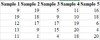
The number of instate players obtained in each set of samples is shown in the below table.

Samples	Number of instate players	Samples	Number of instate players
Sample 1	2	Sample 11	4
Sample 2	1	Sample 12	1
Sample 3	2	Sample 13	3
Sample 4	2	Sample 14	0
Sample 5	1	Sample 15	2
Sample 6	0	Sample 16	0
Sample 7	3	Sample 17	3
Sample 8	3	Sample 18	2
Sample 9	1	Sample 19	3
Sample 10	4	Sample 20	3

Explanation of Solution

Calculation:

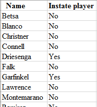
Step 1: In the Excel spreadsheet, write the name of the students and whether they are instate players or not. The snapshot is shown below:

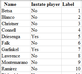
Step 2: Label each of the students using the numbers $1,2,\cdots ,20$. The snapshot is shown below:

Step 3: Use the formula $=\text{RANDBETWEN}\left(\text{Bottom, Top}\right)$ to generate a single set of sample of size 5. Specify the “bottom” value as 1 and “top” value as 20 because there are 20 students. Discard the number if the same number is repeated after appearing once. Repeat the process to generate 20 set of random sample of size 5. The partial snapshot of the chosen random numbers is shown below:

To find the number of instate players in each sample, the label of each instate players are matched with the obtained random number of each set of sample and calculate the number of instate players. The number of instate players obtained in each set of samples are shown in the below table.

Samples	Number of instate players	Samples	Number of instate players
Sample 1	2	Sample 11	4
Sample 2	1	Sample 12	1
Sample 3	2	Sample 13	3
Sample 4	2	Sample 14	0
Sample 5	1	Sample 15	2
Sample 6	0	Sample 16	0
Sample 7	3	Sample 17	3
Sample 8	3	Sample 18	2
Sample 9	1	Sample 19	3
Sample 10	4	Sample 20	3

Section 2:

To determine

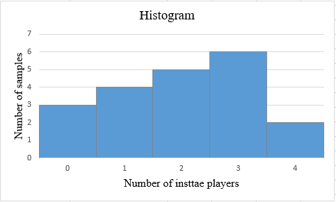
To graph: The histogram for the number of instate players in each set of sample.

Answer to Problem 14E

Solution: The obtained histogram is obtained as:

Explanation of Solution

Graph:

To obtain the histogram for the obtained result in previous part, Excel is used. The below steps are followed to obtained the required histogram.

Step 1: The number of instate players varies from 0 to 4. The number of samples are calculated corresponding to each number of instate players. The number of samples with same number of instate players are clustered. The snapshot of the obtained table is shown below:

Number of instate players members	Number of samples
0	3
1	4
2	5
3	6
4	2

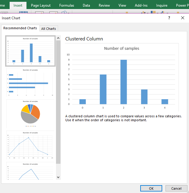
Step 2: Select the data set and go to insert and select the option of cluster column under the Recommended Charts. The screenshot is shown below:

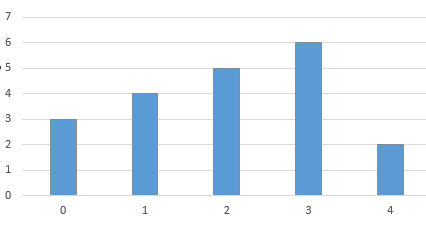
Step 3: Click on OK. The diagram is obtained as:

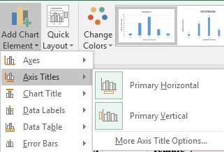
Step 4: Click on the chart area and select the option of “Primary Horizontal” and “Primary Vertical” axis under the “Add Chart Element” to add the axis title. The screenshot is shown below:

Step 5: Click on the bars of the diagrams and reduce the gap width to zero under the “Format Data Series” tab. The screenshot is shown below:

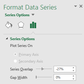
The obtained histogram is:

Section 3:

To determine

To find: The average number of instate players in 20 samples.

Answer to Problem 14E

Solution: The average number of instate players is 2.

Explanation of Solution

Explanation

Calculation:

The average number of instate players can be obtained by using the formula:

$\text{Average}=\frac{\text{Sum of}\left(\text{Number of instate players}\times \text{Number of samples}\right)}{\text{Total number of samples}}$

Hence, the average number of instate players is calculated as:

$\begin{array}{c}\text{Average}=\frac{\text{Sum of}\left(\text{Number of instate players}\times \text{Number of samples}\right)}{\text{Total number of samples}}\\ =\frac{\left(0\times 3\right)+\left(1\times 4\right)+\left(2\times 5\right)+\left(3\times 6\right)+\left(4\times 2\right)}{20}\\ =\frac{0+4+10+18+8}{20}\\ =2\end{array}$

(b)

To determine

To explain: Whether the college should be doubtful about the discrimination if any of the five scholarships does not received by instate players.

Answer to Problem 14E

Solution: The college should suspect the discrimination if any of the five scholarships does not received by instate players.

Explanation of Solution

The event is going to be suspected if the chance of occurrence of that event is approximately 0.05 or less. In the provided scenario, there will be three cases, where the set of samples does not contain any instate players. As the chance is very low, the college can suspect about the discrimination if any of the five scholarships does not receive by instate players.