
Concept explainers
Videos
(a)
Section 1:
The 20 simple random samples of size 5 and record the number of females in each sample.
(a)
Section 1:
Answer to Problem 13E
Solution: The partial output of the 20 simple random samples is shown below:
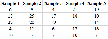
The number of females in each sample is shown below.
| Samples | Number of females | Samples | Number of females |
| Sample 1 | 2 | Sample 11 | 1 |
| Sample 2 | 1 | Sample 12 | 2 |
| Sample 3 | 2 | Sample 13 | 4 |
| Sample 4 | 3 | Sample 14 | 2 |
| Sample 5 | 1 | Sample 15 | 3 |
| Sample 6 | 2 | Sample 16 | 2 |
| Sample 7 | 3 | Sample 17 | 0 |
| Sample 8 | 1 | Sample 18 | 2 |
| Sample 9 | 1 | Sample 19 | 1 |
| Sample 10 | 2 | Sample 20 | 2 |
Explanation of Solution
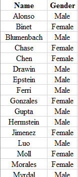
Step 1: Write the name and the gender of the club members in the Excel spreadsheet. The snapshot is shown below:
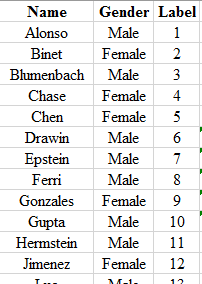
Step 2: Label each of the members using the numbers
Step 3: Use the formula

To find the number of female in each sample, the label of each female member is matched with the obtained random number of each set of sample and then the number of female is counted. The number of females obtained in each set of samples are shown in the below table.
| Samples | Number of females | Samples | Number of females |
| Sample 1 | 2 | Sample 11 | 1 |
| Sample 2 | 1 | Sample 12 | 2 |
| Sample 3 | 2 | Sample 13 | 4 |
| Sample 4 | 3 | Sample 14 | 2 |
| Sample 5 | 1 | Sample 15 | 3 |
| Sample 6 | 2 | Sample 16 | 2 |
| Sample 7 | 3 | Sample 17 | 0 |
| Sample 8 | 1 | Sample 18 | 2 |
| Sample 9 | 1 | Sample 19 | 1 |
| Sample 10 | 2 | Sample 20 | 2 |
To graph: The histogram for the number of females in each set of sample.
Explanation of Solution
Graph: To obtain the histogram for the obtained result in previous part, Excel is used. The below steps are followed to obtain the required histogram.
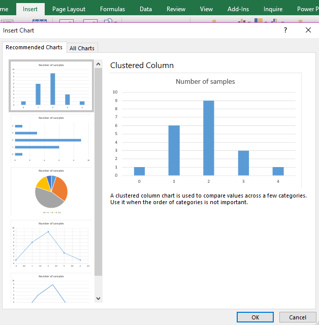
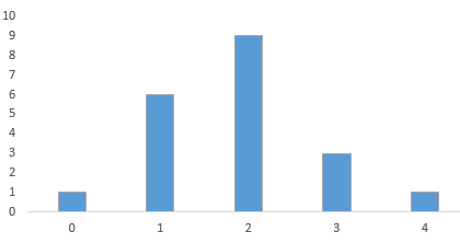
Step 1: The number of females varies from 0 to 4. The number of samples are calculated corresponding to each number of females. The number of samples with the same number of female members is clustered. The snapshot of the obtained table is shown below:
| Number of female members | Number of samples |
| 0 | 1 |
| 1 | 6 |
| 2 | 9 |
| 3 | 3 |
| 4 | 1 |
Step 2: Select the data set and go to insert and select the option of cluster column under the Recommended Charts. The screenshot is shown below:
Step 3: Click on OK. The diagram is obtained as:
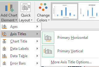
Step 4: Click on the chart area and select the option of “Primary Horizontal” and “Primary Vertical” axis under the “Add Chart Element” to add the axis title. The screenshot is shown below:
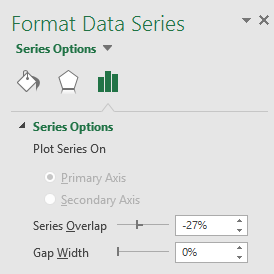
Step 5: Click on the bars of the diagrams and reduce the gap width to zero under the “Format Data Series” tab. The screenshot is shown below:
The obtained histogram is:
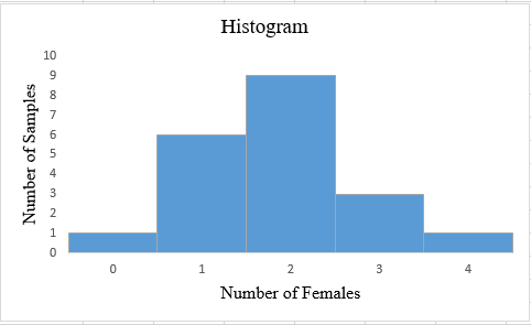
Interpretation: The obtained histogram for the number of females in each set of sample follows
To find: The average number of females in 20 samples.
Answer to Problem 13E
Solution: The average number of female is 1.85.
Explanation of Solution
Calculation:
The average number of females can be obtained by using the formula:
Hence, the average number of females is calculated as:
Therefore, the average number of females in 20 samples is 1.85.
(b)
To explain: Whether the club members should be doubtful about the discrimination if any of the five tickets does not received by women.
(b)
Answer to Problem 13E
Solution: The club member should suspect the discrimination if any of the five tickets does not received by women.
Explanation of Solution
Want to see more full solutions like this?
Chapter 3 Solutions
Loose-leaf Version for Statistics: Concepts and Controversies


- This problem is based on the fundamental option pricing formula for the continuous-time model developed in class, namely the value at time 0 of an option with maturity T and payoff F is given by: We consider the two options below: Fo= -rT = e Eq[F]. 1 A. An option with which you must buy a share of stock at expiration T = 1 for strike price K = So. B. An option with which you must buy a share of stock at expiration T = 1 for strike price K given by T K = T St dt. (Note that both options can have negative payoffs.) We use the continuous-time Black- Scholes model to price these options. Assume that the interest rate on the money market is r. (a) Using the fundamental option pricing formula, find the price of option A. (Hint: use the martingale properties developed in the lectures for the stock price process in order to calculate the expectations.) (b) Using the fundamental option pricing formula, find the price of option B. (c) Assuming the interest rate is very small (r ~0), use Taylor…arrow_forwardDiscuss and explain in the picturearrow_forwardBob and Teresa each collect their own samples to test the same hypothesis. Bob’s p-value turns out to be 0.05, and Teresa’s turns out to be 0.01. Why don’t Bob and Teresa get the same p-values? Who has stronger evidence against the null hypothesis: Bob or Teresa?arrow_forward
- Review a classmate's Main Post. 1. State if you agree or disagree with the choices made for additional analysis that can be done beyond the frequency table. 2. Choose a measure of central tendency (mean, median, mode) that you would like to compute with the data beyond the frequency table. Complete either a or b below. a. Explain how that analysis can help you understand the data better. b. If you are currently unable to do that analysis, what do you think you could do to make it possible? If you do not think you can do anything, explain why it is not possible.arrow_forward0|0|0|0 - Consider the time series X₁ and Y₁ = (I – B)² (I – B³)Xt. What transformations were performed on Xt to obtain Yt? seasonal difference of order 2 simple difference of order 5 seasonal difference of order 1 seasonal difference of order 5 simple difference of order 2arrow_forwardCalculate the 90% confidence interval for the population mean difference using the data in the attached image. I need to see where I went wrong.arrow_forward
- Microsoft Excel snapshot for random sampling: Also note the formula used for the last column 02 x✓ fx =INDEX(5852:58551, RANK(C2, $C$2:$C$51)) A B 1 No. States 2 1 ALABAMA Rand No. 0.925957526 3 2 ALASKA 0.372999976 4 3 ARIZONA 0.941323044 5 4 ARKANSAS 0.071266381 Random Sample CALIFORNIA NORTH CAROLINA ARKANSAS WASHINGTON G7 Microsoft Excel snapshot for systematic sampling: xfx INDEX(SD52:50551, F7) A B E F G 1 No. States Rand No. Random Sample population 50 2 1 ALABAMA 0.5296685 NEW HAMPSHIRE sample 10 3 2 ALASKA 0.4493186 OKLAHOMA k 5 4 3 ARIZONA 0.707914 KANSAS 5 4 ARKANSAS 0.4831379 NORTH DAKOTA 6 5 CALIFORNIA 0.7277162 INDIANA Random Sample Sample Name 7 6 COLORADO 0.5865002 MISSISSIPPI 8 7:ONNECTICU 0.7640596 ILLINOIS 9 8 DELAWARE 0.5783029 MISSOURI 525 10 15 INDIANA MARYLAND COLORADOarrow_forwardSuppose the Internal Revenue Service reported that the mean tax refund for the year 2022 was $3401. Assume the standard deviation is $82.5 and that the amounts refunded follow a normal probability distribution. Solve the following three parts? (For the answer to question 14, 15, and 16, start with making a bell curve. Identify on the bell curve where is mean, X, and area(s) to be determined. 1.What percent of the refunds are more than $3,500? 2. What percent of the refunds are more than $3500 but less than $3579? 3. What percent of the refunds are more than $3325 but less than $3579?arrow_forwardA normal distribution has a mean of 50 and a standard deviation of 4. Solve the following three parts? 1. Compute the probability of a value between 44.0 and 55.0. (The question requires finding probability value between 44 and 55. Solve it in 3 steps. In the first step, use the above formula and x = 44, calculate probability value. In the second step repeat the first step with the only difference that x=55. In the third step, subtract the answer of the first part from the answer of the second part.) 2. Compute the probability of a value greater than 55.0. Use the same formula, x=55 and subtract the answer from 1. 3. Compute the probability of a value between 52.0 and 55.0. (The question requires finding probability value between 52 and 55. Solve it in 3 steps. In the first step, use the above formula and x = 52, calculate probability value. In the second step repeat the first step with the only difference that x=55. In the third step, subtract the answer of the first part from the…arrow_forward
- If a uniform distribution is defined over the interval from 6 to 10, then answer the followings: What is the mean of this uniform distribution? Show that the probability of any value between 6 and 10 is equal to 1.0 Find the probability of a value more than 7. Find the probability of a value between 7 and 9. The closing price of Schnur Sporting Goods Inc. common stock is uniformly distributed between $20 and $30 per share. What is the probability that the stock price will be: More than $27? Less than or equal to $24? The April rainfall in Flagstaff, Arizona, follows a uniform distribution between 0.5 and 3.00 inches. What is the mean amount of rainfall for the month? What is the probability of less than an inch of rain for the month? What is the probability of exactly 1.00 inch of rain? What is the probability of more than 1.50 inches of rain for the month? The best way to solve this problem is begin by a step by step creating a chart. Clearly mark the range, identifying the…arrow_forwardClient 1 Weight before diet (pounds) Weight after diet (pounds) 128 120 2 131 123 3 140 141 4 178 170 5 121 118 6 136 136 7 118 121 8 136 127arrow_forwardClient 1 Weight before diet (pounds) Weight after diet (pounds) 128 120 2 131 123 3 140 141 4 178 170 5 121 118 6 136 136 7 118 121 8 136 127 a) Determine the mean change in patient weight from before to after the diet (after – before). What is the 95% confidence interval of this mean difference?arrow_forward
 MATLAB: An Introduction with ApplicationsStatisticsISBN:9781119256830Author:Amos GilatPublisher:John Wiley & Sons Inc
 Probability and Statistics for Engineering and th...StatisticsISBN:9781305251809Author:Jay L. DevorePublisher:Cengage Learning
 Statistics for The Behavioral Sciences (MindTap C...StatisticsISBN:9781305504912Author:Frederick J Gravetter, Larry B. WallnauPublisher:Cengage Learning
 Elementary Statistics: Picturing the World (7th E...StatisticsISBN:9780134683416Author:Ron Larson, Betsy FarberPublisher:PEARSON
 The Basic Practice of StatisticsStatisticsISBN:9781319042578Author:David S. Moore, William I. Notz, Michael A. FlignerPublisher:W. H. Freeman
 Introduction to the Practice of StatisticsStatisticsISBN:9781319013387Author:David S. Moore, George P. McCabe, Bruce A. CraigPublisher:W. H. Freeman