Chapter 2R, Problem 3FRQ

a)

To determine

The question requires us to draw the supply and demand diagram for sandals and mark or label the equilibrium price and quantity in the market.

Explanation of Solution

In the market for sandals, S1 shows the supply curve, and D1 represents the demand curve for sandals. The intersection point of the supply and demand curve gives the equilibrium state in the market.

At equilibrium,

Quantity supplied = Quantity demanded = Q1 units.

The following graph represents the market for sandals:

  

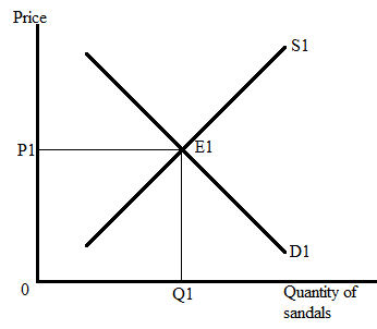
Here, E1 represents the equilibrium point where the supply curve and demand curve intersect each other. The equilibrium quantity is Q1, and the equilibrium price is P1.

b)

To determine

The question requires us to illustrate the impact of higher income on the equilibrium price and quantity of sandals when sandals are normal goods and label the new equilibrium price and quantity.

Explanation of Solution

The following graph represents the impact of higher income on the equilibrium price and quantity of the sandals:

  

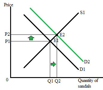
Here, E1 represents the initial equilibrium state in the sandal market, where Q1 is the equilibrium quantity, and P1 is the equilibrium price. Since sandals are normal goods, an increase in the income of consumers will cause the demand for sandals to increase.

A higher demand causes the demand curve to shift rightward from D1 to D2, and results in a higher price (P2) and higher quantity (Q2). 

E2 represents the new equilibrium point where P2 is the new market price for the sandals and Q2 represents the new equilibrium quantity of the sandals.

Economics Concept Introduction

An increase in income level will lead to a higher demand for normal goods.

c)

To determine

The question requires us to illustrate the impact of higher income and higher wages on the equilibrium quantity and compare the result with the initial equilibrium price and quantity.

Explanation of Solution

The simultaneous increase in consumers’ income and workers’ wages will increase the price level of sandals, but the impact on equilibrium quantity will depend on the magnitude of change in supply and demand of the sandals so the result will be ambiguous.

Here, three outcomes are possible depending on the magnitude of change in supply and demand:

1. When a change in supply is more than the change in demand, the market quantity will fall below the initial equilibrium level (Q3 < Q1
2. When a change in supply is less than the change in demand, the market quantity will fall but stay above the initial equilibrium level of quantity (Q1
3. When a change in supply is equal to the change in demand, the new market quantity will be equal to the initial equilibrium level of quantity (Q1=Q3

The following graph represents ‘situation 3’ and the combined impact of higher income and higher wages in the market for sandals:

  

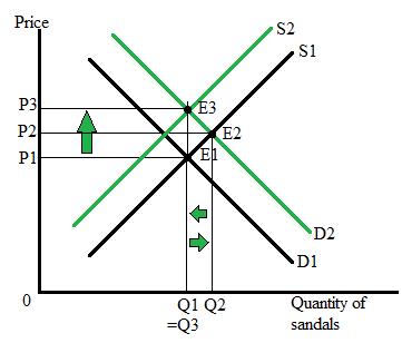
Here, E1 is the initial equilibrium level where P1 is the equilibrium price, and Q1 is the equilibrium quantity. Due to an increase in income level demand for sandals rises from D1 and D2 and causes the price and quantity of sandals to rise. At the same time, an increase in the wage of the sandal-making workers cause the input costs to rise and thus discourages the producer from producing less quantity of the sandals. As a result of higher input costs, the supply of sandals falls and causes the supply curve to shift leftward from S1 to S2.

Finally, the economy reaches new equilibrium point E3 where the market price increases from P1 to P3, and equilibrium quantity falls back to the initial level Q1.