Concept explainers
Videos
To calculate: The temperature on the heated plate with fixed temperature at the boundaries and round corners at upper right and lower left corners; considering the value of weighing factor for overrelaxation as 1.5 and performing iteration up to
Answer to Problem 7P
Solution:
Heated plate having rounded upper right and lower left corners has the temperature distribution with the desired level of accuracy as,
Explanation of Solution
Given Information:
The fixed temperature at top and right boundary is
For overrelaxation the weighing factor is 1.5.
Limiting condition for iteration is
Formula used:
For a square grid, that is,
With
Overrelaxation is applied using the following expression after each iteration,
In the above expression,
The percent relative error is calculated using the following expression,
Laplacian equation for a node adjacent to an irregular boundary is solved for temperature distribution as,
Calculation:
Consider,
Consider the value of the parameters as,
The temperature at the node
Thus,
Further, the temperature at the node
Thus,
Liebmann’s method is used to solve the temperature on the heated plate iteratively in MATLAB, until the percent relative error falls below 1%.
Use the following MATLAB code to implement the Liebmann’s method and the equation at the nodes
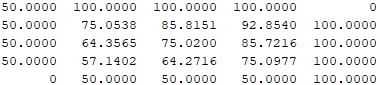
Execute the above code to obtain the temperature distribution and the number of iterations performed, in the output as shown below,
Hence, the temperature on the heated plate with desired accuracy is achieved after 9 iterations as obtained in the above MATLAB output.
Want to see more full solutions like this?
Chapter 29 Solutions
EBK NUMERICAL METHODS FOR ENGINEERS


- This is an exam review question. The answer is Pmin = 622.9 lb but whyarrow_forwardPlease do not use any AI tools to solve this question. I need a fully manual, step-by-step solution with clear explanations, as if it were done by a human tutor. No AI-generated responses, please.arrow_forwardPlease do not use any AI tools to solve this question. I need a fully manual, step-by-step solution with clear explanations, as if it were done by a human tutor. No AI-generated responses, please.arrow_forward
- Please do not use any AI tools to solve this question. I need a fully manual, step-by-step solution with clear explanations, as if it were done by a human tutor. No AI-generated responses, please.arrow_forwardThis is an old practice exam. Fce = 110lb and FBCD = 62 lb but whyarrow_forwardQuiz/An eccentrically loaded bracket is welded to the support as shown in Figure below. The load is static. The weld size for weld w1 is h1 = 4mm, for w2 h2 = 6mm, and for w3 is h3 =6.5 mm. Determine the safety factor (S.f) for the welds. F=29 kN. Use an AWS Electrode type (E100xx). 163 mm S 133 mm 140 mm Please solve the question above I solved the question but I'm sure the answer is wrong the link : https://drive.google.com/file/d/1w5UD2EPDiaKSx3W33aj Rv0olChuXtrQx/view?usp=sharingarrow_forward
- Q2: (15 Marks) A water-LiBr vapor absorption system incorporates a heat exchanger as shown in the figure. The temperatures of the evaporator, the absorber, the condenser, and the generator are 10°C, 25°C, 40°C, and 100°C respectively. The strong liquid leaving the pump is heated to 50°C in the heat exchanger. The refrigerant flow rate through the condenser is 0.12 kg/s. Calculate (i) the heat rejected in the absorber, and (ii) the COP of the cycle. Yo 8 XE-V lo 9 Pc 7 condenser 5 Qgen PG 100 Qabs Pe evaporator PRV 6 PA 10 3 generator heat exchanger 2 pump 185 absorberarrow_forwardQ5:(? Design the duct system of the figure below by using the balanced pressure method. The velocity in the duct attached to the AHU must not exceed 5m/s. The pressure loss for each diffuser is equal to 10Pa. 100CFM 100CFM 100CFM ☑ ☑ 40m AHU -16m- 8m- -12m- 57m 250CFM 40m -14m- 26m 36m ☑ 250CFMarrow_forwardA mass of ideal gas in a closed piston-cylinder system expands from 427 °C and 16 bar following the process law, pv1.36 = Constant (p times v to the power of 1.36 equals to a constant). For the gas, initial : final pressure ratio is 4:1 and the initial gas volume is 0.14 m³. The specific heat of the gas at constant pressure, Cp = 0.987 kJ/kg-K and the specific gas constant, R = 0.267 kJ/kg.K. Determine the change in total internal energy in the gas during the expansion. Enter your numerical answer in the answer box below in KILO JOULES (not in Joules) but do not enter the units. (There is no expected number of decimal points or significant figures).arrow_forward
- my ID# 016948724. Please solve this problem step by steparrow_forwardMy ID# 016948724 please find the forces for Fx=0: fy=0: fz=0: please help me to solve this problem step by steparrow_forwardMy ID# 016948724 please solve the proble step by step find the forces fx=o: fy=0; fz=0; and find shear moment and the bending moment diagran please draw the diagram for the shear and bending momentarrow_forward
 Elements Of ElectromagneticsMechanical EngineeringISBN:9780190698614Author:Sadiku, Matthew N. O.Publisher:Oxford University Press
 Mechanics of Materials (10th Edition)Mechanical EngineeringISBN:9780134319650Author:Russell C. HibbelerPublisher:PEARSON
 Thermodynamics: An Engineering ApproachMechanical EngineeringISBN:9781259822674Author:Yunus A. Cengel Dr., Michael A. BolesPublisher:McGraw-Hill Education
 Control Systems EngineeringMechanical EngineeringISBN:9781118170519Author:Norman S. NisePublisher:WILEY
 Mechanics of Materials (MindTap Course List)Mechanical EngineeringISBN:9781337093347Author:Barry J. Goodno, James M. GerePublisher:Cengage Learning
 Engineering Mechanics: StaticsMechanical EngineeringISBN:9781118807330Author:James L. Meriam, L. G. Kraige, J. N. BoltonPublisher:WILEY