Sub part (a):
Steady state level of output.
Sub part (a):
Explanation of Solution
The steady state level of output is calculated as follows:
The steady state level of output is 200 units.
Concept introduction:
Sub part (b):
Solow diagram to show short run impact.
Sub part (b):
Explanation of Solution
Figure 1 depicts Solow diagram which shows the short run impact of a 21% increase in the amount of labor available.
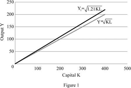
In figure 1, the horizontal axis represents the capital (K) and the vertical axis represents the output (Y). The initial production function
Concept introduction:
Economic growth: The economic growth is the increase in the overall goods and services produced per head in the economy over a specific period of time.
Solow growth rate The Solow growth rate is the rate of economic growth with given flexible price, and the existing real factors of capita, labor and knowledge. The Solow growth rate is an economy’s potential growth rate.
Sub part (c):
Steady state level of output.
Sub part (c):
Explanation of Solution
The new steady state level of output is calculated as follows:
The new steady state level of output is 220 units.
Concept introduction:
Economic growth: The economic growth is the increase in the overall goods and services produced per head in the economy over a specific period of time.
Sub part (d):
The new steady state level of output in the diagram.
Sub part (d):
Explanation of Solution
The new steady state level of output is 220 units which is depicted in the figure 1.
Sub part (e):
Action to gain long lasting benefits from the increase in capital stock.
Sub part (e):
Explanation of Solution
The initial production function is algebraically represented as follows:
Squaring both sides,
And solving for K, we get
Substitute K into the steady-state condition
And solve for Y by multiplying L and dividing by
Similarly, the new production function can be algebraically represented as follows:
Substitute K into the steady-state condition
And solve for Y by multiplying L and dividing by
Equating (1) in (2) we get
Substituting the values in equation (3) we get
Further, the percentage change in the output is depicted as follows:
This implies the steady-state level of output will grow by 21% per cent in the long run.
Concept introduction:
Production function: It is the relationship between the inputs employed by a firm and the maximum output the firm can produce with those inputs.
Sub part (f):
Output per worker.
Sub part (f):
Explanation of Solution
The output per worker in the initial steady state is calculated as follows:
The output per worker in the initial steady state is 2 units per labor.
The output per worker in the short run is calculated as follows:
The output per worker in short run is 1.82 units per labor.
The output per worker in the initial steady state is calculated as follows:
The output per worker in the long run is 2 units per labor.
Sub part (g):
New immigration policy and its effect.
Sub part (g):
Explanation of Solution
The citizens of the country are neither made worse off nor better off in the long run by a new immigration policy. This is because the new long-run level of output per worker compare with the initial level of output per worker remains unchanged which is 2 units per labor. This is unlike the short run effect which has lower output per worker. In the long run, the steady output level is determined largely by the
Concept introduction:
Depreciation: Depreciation is the process of decreasing the value of an asset over time especially due to wear and tear.
Investment: The investment is the money invests in terms of assets and building by the individual for the future consumption and profit making.
Sub part (h):
New steady state level of capital.
Sub part (h):
Explanation of Solution
The new steady state level of capital is calculated as follows
We know
Also
Equating all these we get,
Substituting the values we get
Thus the new steady state level of capital is 484, so that
Want to see more full solutions like this?
Chapter 28 Solutions
Modern Principles of Economics

- In the graph at the right, the average variable cost is curve ☐. The average total cost is curve marginal cost is curve The C Cost per Unit ($) Per Unit Costs A 0 Output Quantity Barrow_forwardWhat are some of the question s that I can ask my economic teacher?arrow_forwardAnswer question 2 only.arrow_forward
- 1. A pension fund manager is considering three mutual funds. The first is a stock fund, the second is a long-term government and corporate fund, and the third is a (riskless) T-bill money market fund that yields a rate of 8%. The probability distributions of the risky funds have the following characteristics: Standard Deviation (%) Expected return (%) Stock fund (Rs) 20 30 Bond fund (RB) 12 15 The correlation between the fund returns is .10.arrow_forwardFrederick Jones operates a sole proprietorship business in Trinidad and Tobago. His gross annual revenue in 2023 was $2,000,000. He wants to register for VAT, but he is unsure of what VAT entails, the requirements for registration and what he needs to do to ensure that he is fully compliant with VAT regulations. Make reference to the Vat Act of Trinidad and Tobago and explain to Mr. Jones what VAT entails, the requirements for registration and the requirements to be fully compliant with VAT regulations.arrow_forwardCan you show me the answers for parts a and b? Thanks.arrow_forward
- What are the answers for parts a and b? Thanksarrow_forwardWhat are the answers for a,b,c,d? Are they supposed to be numerical answers or in terms of a variable?arrow_forwardSue is a sole proprietor of her own sewing business. Revenues are $150,000 per year and raw material (cloth, thread) costs are $130,000 per year. Sue pays herself a salary of $60,000 per year but gave up a job with a salary of $80,000 to run the business. ○ A. Her accounting profits are $0. Her economic profits are - $60,000. ○ B. Her accounting profits are $0. Her economic profits are - $40,000. ○ C. Her accounting profits are - $40,000. Her economic profits are - $60,000. ○ D. Her accounting profits are - $60,000. Her economic profits are -$40,000.arrow_forward
- Select a number that describes the type of firm organization indicated. Descriptions of Firm Organizations: 1. has one owner-manager who is personally responsible for all aspects of the business, including its debts 2. one type of partner takes part in managing the firm and is personally liable for the firm's actions and debts, and the other type of partner takes no part in the management of the firm and risks only the money that they have invested 3. owners are not personally responsible for anything that is done in the name of the firm 4. owned by the government but is usually under the direction of a more or less independent, state-appointed board 5. established with the explicit objective of providing goods or services but only in a manner that just covers its costs 6. has two or more joint owners, each of whom is personally responsible for all of the partnership's debts Type of Firm Organization a. limited partnership b. single proprietorship c. corporation Correct Numberarrow_forwardThe table below provides the total revenues and costs for a small landscaping company in a recent year. Total Revenues ($) 250,000 Total Costs ($) - wages and salaries 100,000 -risk-free return of 2% on owner's capital of $25,000 500 -interest on bank loan 1,000 - cost of supplies 27,000 - depreciation of capital equipment 8,000 - additional wages the owner could have earned in next best alternative 30,000 -risk premium of 4% on owner's capital of $25,000 1,000 The economic profits for this firm are ○ A. $83,000. B. $82,500. OC. $114,000. OD. $83,500. ○ E. $112,500.arrow_forwardOutput TFC ($) TVC ($) TC ($) (Q) 2 100 104 204 3 100 203 303 4 100 300 400 5 100 405 505 6 100 512 612 7 100 621 721 Given the information about short-run costs in the table above, we can conclude that the firm will minimize the average total cost of production when Q = (Round your response to the nearest whole number.)arrow_forward

 Principles of Economics (12th Edition)EconomicsISBN:9780134078779Author:Karl E. Case, Ray C. Fair, Sharon E. OsterPublisher:PEARSON
 Engineering Economy (17th Edition)EconomicsISBN:9780134870069Author:William G. Sullivan, Elin M. Wicks, C. Patrick KoellingPublisher:PEARSON
 Principles of Economics (MindTap Course List)EconomicsISBN:9781305585126Author:N. Gregory MankiwPublisher:Cengage Learning
 Managerial Economics: A Problem Solving ApproachEconomicsISBN:9781337106665Author:Luke M. Froeb, Brian T. McCann, Michael R. Ward, Mike ShorPublisher:Cengage Learning
 Managerial Economics & Business Strategy (Mcgraw-...EconomicsISBN:9781259290619Author:Michael Baye, Jeff PrincePublisher:McGraw-Hill Education