
(a)
To make a
(a)
Answer to Problem 28.37E
Yes, the graph suggest that a multiple regression might be appropriate.
Explanation of Solution
In the question, it is given that an experiment compared the effects of adding various amounts of nitrogen fertilizers to two genotypes of tomato plants, a mild-type and a mutant variety. The percent of phosphorus in the plant, nitrogen and genotype is given in a table. Thus, the scatterplot of the amount of phosphorus in the plant against nitrogen, using different symbols for the two plant genotype is as follows:
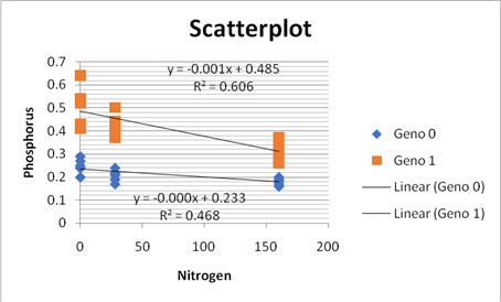
In the scatterplot, we can see that the genotype zero is in red color and genotype one is in blue color. And the lines in the scatterplot are almost parallel so it is linear in nature and in both the lines the points are moving downwards so they are negative in relationship. Thus, as they are parallel so the graph suggest that a multiple regression might be appropriate for these data.
(b)
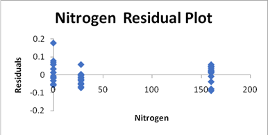
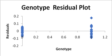
To use a software to obtain the estimated multiple linear regression equation when the two explanatory variables nitrogen and genotype are included and create a residual plot and explain are the conditions for multiple linear regression satisfied.
(b)
Answer to Problem 28.37E
The estimated multiple linear regression equation is
Explanation of Solution
In the question, it is given that an experiment compared the effects of adding various amounts of nitrogen fertilizers to two genotypes of tomato plants, a mild-type and a mutant variety. The percent of phosphorus in the plant, nitrogen and genotype is given in a table. Now, we will use the Excel to obtain the estimated multiple linear regression equation when the two explanatory variables nitrogen and genotype are included and also the residual plot is constructed. We will use the option data analysis in the data tab and run the
| ANOVA | |||||
| df | SS | MS | F | Significance F | |
| Regression | 2 | 0.46916 | 0.23458 | 76.2375 | 4.25E-13 |
| Residual | 33 | 0.10154 | 0.003077 | ||
| Total | 35 | 0.5707 |
| Coefficients | Standard Error | t Stat | P-value | |
| Intercept | 0.256853 | 0.015489 | 16.58326 | 1.43E-17 |
| Nitrogen | -0.00071 | 0.000133 | -5.37461 | 6.11E-06 |
| Genotype | 0.205556 | 0.01849 | 11.11704 | 1.07E-12 |
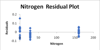
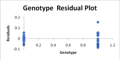
The residual plot will be constructed as:
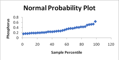
And the normal plot will be constructed as:
Now, the estimated multiple linear regression equation when the two explanatory variables nitrogen and genotype are included is as:
Where
(c)
To create a new variable called interaction by multiplying the explanatory variables nitrogen and genotype and add this new variable to your regression model and provide the estimated multiple linear regression equation and create regression plot for this and discuss whether the conditions for multiple linear regression are met.
(c)
Answer to Problem 28.37E
The conditions for multiple linear regression are met and the estimated multiple linear regression equation is
Explanation of Solution
In the question, it is given that an experiment compared the effects of adding various amounts of nitrogen fertilizers to two genotypes of tomato plants, a mild-type and a mutant variety. The percent of phosphorus in the plant, nitrogen and genotype is given in a table. And a new variable called interaction is created by multiplying the explanatory variables nitrogen and genotype. Now, we will use the Excel to obtain the estimated multiple linear regression equation when the two explanatory variables nitrogen and genotype and the interaction are included and also the residual plot is constructed. We will use the option data analysis in the data tab and run the regression analysis. The result will be as:
| ANOVA | |||||
| df | SS | MS | F | Significance F | |
| Regression | 3 | 0.49273 | 0.164243 | 67.4079 | 6.35E-14 |
| Residual | 32 | 0.07797 | 0.002437 | ||
| Total | 35 | 0.5707 |
| Coefficients | Standard Error | t Stat | P-value | |
| Intercept | 0.23387 | 0.015639 | 14.95438 | 5.42E-16 |
| Nitrogen | -0.00035 | 0.000167 | -2.0715 | 0.046455 |
| Genotype | 0.251522 | 0.022117 | 11.37245 | 8.91E-13 |
| Interaction | -0.00073 | 0.000236 | -3.11022 | 0.003912 |
The residual plot is as follows:
The normal plot is as follows:

Now, the estimated multiple linear regression equation when the two explanatory variables nitrogen and genotype and interaction are included is as:
Where
(d)
To explain does the ANOVA table for the model with the interaction term indicate that at least one of the explanatory variables is helpful in predicting the amount of phosphorus in the plant and explain do the individual t tests indicate that all coefficients are significantly different from zero.
(d)
Answer to Problem 28.37E
Yes, the ANOVA table for the model with the interaction term indicates that at least one of the explanatory variables is helpful in predicting the amount of phosphorus in the plant and the individual t tests indicate that all coefficients are significantly different from zero.
Explanation of Solution
In the question, it is given that an experiment compared the effects of adding various amounts of nitrogen fertilizers to two genotypes of tomato plants, a mild-type and a mutant variety. The percent of phosphorus in the plant, nitrogen and genotype is given in a table. Since in the ANOVA table in part (c) we can see that the P-value is less than the level of significance,
Thus, we can say that the ANOVA table for the model with the interaction term indicates that at least one of the explanatory variables is helpful in predicting the amount of phosphorus in the plant. And as we can see in the result of the regression analysis in part (c), we can see that all the P-values are less than the level of significance i.e.
Thus, we have sufficient evidence to conclude that the individual t tests indicate that all coefficients are significantly different from zero.
Want to see more full solutions like this?
Chapter 28 Solutions
PRACT STAT W/ ACCESS 6MO LOOSELEAF

- Please help me answer the following questions from this problem.arrow_forwardPlease help me find the sample variance for this question.arrow_forwardCrumbs Cookies was interested in seeing if there was an association between cookie flavor and whether or not there was frosting. Given are the results of the last week's orders. Frosting No Frosting Total Sugar Cookie 50 Red Velvet 66 136 Chocolate Chip 58 Total 220 400 Which category has the greatest joint frequency? Chocolate chip cookies with frosting Sugar cookies with no frosting Chocolate chip cookies Cookies with frostingarrow_forward
- The table given shows the length, in feet, of dolphins at an aquarium. 7 15 10 18 18 15 9 22 Are there any outliers in the data? There is an outlier at 22 feet. There is an outlier at 7 feet. There are outliers at 7 and 22 feet. There are no outliers.arrow_forwardStart by summarizing the key events in a clear and persuasive manner on the article Endrikat, J., Guenther, T. W., & Titus, R. (2020). Consequences of Strategic Performance Measurement Systems: A Meta-Analytic Review. Journal of Management Accounting Research?arrow_forwardThe table below was compiled for a middle school from the 2003 English/Language Arts PACT exam. Grade 6 7 8 Below Basic 60 62 76 Basic 87 134 140 Proficient 87 102 100 Advanced 42 24 21 Partition the likelihood ratio test statistic into 6 independent 1 df components. What conclusions can you draw from these components?arrow_forward
- What is the value of the maximum likelihood estimate, θ, of θ based on these data? Justify your answer. What does the value of θ suggest about the value of θ for this biased die compared with the value of θ associated with a fair, unbiased, die?arrow_forwardShow that L′(θ) = Cθ394(1 −2θ)604(395 −2000θ).arrow_forwarda) Let X and Y be independent random variables both with the same mean µ=0. Define a new random variable W = aX +bY, where a and b are constants. (i) Obtain an expression for E(W).arrow_forward
- The table below shows the estimated effects for a logistic regression model with squamous cell esophageal cancer (Y = 1, yes; Y = 0, no) as the response. Smoking status (S) equals 1 for at least one pack per day and 0 otherwise, alcohol consumption (A) equals the average number of alcohoic drinks consumed per day, and race (R) equals 1 for blacks and 0 for whites. Variable Effect (β) P-value Intercept -7.00 <0.01 Alcohol use 0.10 0.03 Smoking 1.20 <0.01 Race 0.30 0.02 Race × smoking 0.20 0.04 Write-out the prediction equation (i.e., the logistic regression model) when R = 0 and again when R = 1. Find the fitted Y S conditional odds ratio in each case. Next, write-out the logistic regression model when S = 0 and again when S = 1. Find the fitted Y R conditional odds ratio in each case.arrow_forwardThe chi-squared goodness-of-fit test can be used to test if data comes from a specific continuous distribution by binning the data to make it categorical. Using the OpenIntro Statistics county_complete dataset, test the hypothesis that the persons_per_household 2019 values come from a normal distribution with mean and standard deviation equal to that variable's mean and standard deviation. Use signficance level a = 0.01. In your solution you should 1. Formulate the hypotheses 2. Fill in this table Range (-⁰⁰, 2.34] (2.34, 2.81] (2.81, 3.27] (3.27,00) Observed 802 Expected 854.2 The first row has been filled in. That should give you a hint for how to calculate the expected frequencies. Remember that the expected frequencies are calculated under the assumption that the null hypothesis is true. FYI, the bounderies for each range were obtained using JASP's drag-and-drop cut function with 8 levels. Then some of the groups were merged. 3. Check any conditions required by the chi-squared…arrow_forwardSuppose that you want to estimate the mean monthly gross income of all households in your local community. You decide to estimate this population parameter by calling 150 randomly selected residents and asking each individual to report the household’s monthly income. Assume that you use the local phone directory as the frame in selecting the households to be included in your sample. What are some possible sources of error that might arise in your effort to estimate the population mean?arrow_forward
 MATLAB: An Introduction with ApplicationsStatisticsISBN:9781119256830Author:Amos GilatPublisher:John Wiley & Sons Inc
 Probability and Statistics for Engineering and th...StatisticsISBN:9781305251809Author:Jay L. DevorePublisher:Cengage Learning
 Statistics for The Behavioral Sciences (MindTap C...StatisticsISBN:9781305504912Author:Frederick J Gravetter, Larry B. WallnauPublisher:Cengage Learning
 Elementary Statistics: Picturing the World (7th E...StatisticsISBN:9780134683416Author:Ron Larson, Betsy FarberPublisher:PEARSON
 The Basic Practice of StatisticsStatisticsISBN:9781319042578Author:David S. Moore, William I. Notz, Michael A. FlignerPublisher:W. H. Freeman
 Introduction to the Practice of StatisticsStatisticsISBN:9781319013387Author:David S. Moore, George P. McCabe, Bruce A. CraigPublisher:W. H. Freeman