(a)
To make a
(a)
Answer to Problem 28.37E
Yes, the graph suggest that a multiple regression might be appropriate.
Explanation of Solution
In the question, it is given that an experiment compared the effects of adding various amounts of nitrogen fertilizers to two genotypes of tomato plants, a mild-type and a mutant variety. The percent of phosphorus in the plant, nitrogen and genotype is given in a table. Thus, the scatterplot of the amount of phosphorus in the plant against nitrogen, using different symbols for the two plant genotype is as follows:
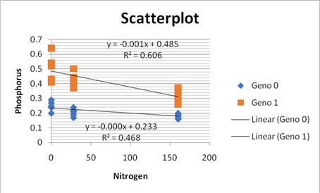
In the scatterplot, we can see that the genotype zero is in red color and genotype one is in blue color. And the lines in the scatterplot are almost parallel so it is linear in nature and in both the lines the points are moving downwards so they are negative in relationship. Thus, as they are parallel so the graph suggest that a multiple regression might be appropriate for these data.
(b)
To use a software to obtain the estimated multiple linear regression equation when the two explanatory variables nitrogen and genotype are included and create a residual plot and explain are the conditions for multiple linear regression satisfied.
(b)
Answer to Problem 28.37E
The estimated multiple linear regression equation is
Explanation of Solution
In the question, it is given that an experiment compared the effects of adding various amounts of nitrogen fertilizers to two genotypes of tomato plants, a mild-type and a mutant variety. The percent of phosphorus in the plant, nitrogen and genotype is given in a table. Now, we will use the Excel to obtain the estimated multiple linear regression equation when the two explanatory variables nitrogen and genotype are included and also the residual plot is constructed. We will use the option data analysis in the data tab and run the
| ANOVA | |||||
| df | SS | MS | F | Significance F | |
| Regression | 2 | 0.46916 | 0.23458 | 76.2375 | 4.25E-13 |
| Residual | 33 | 0.10154 | 0.003077 | ||
| Total | 35 | 0.5707 |
| Coefficients | Standard Error | t Stat | P-value | |
| Intercept | 0.256853 | 0.015489 | 16.58326 | 1.43E-17 |
| Nitrogen | -0.00071 | 0.000133 | -5.37461 | 6.11E-06 |
| Genotype | 0.205556 | 0.01849 | 11.11704 | 1.07E-12 |
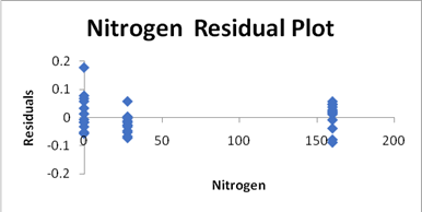
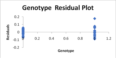
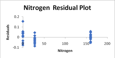
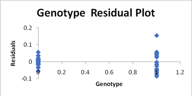
The residual plot will be constructed as:
And the normal plot will be constructed as:
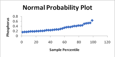
Now, the estimated multiple linear regression equation when the two explanatory variables nitrogen and genotype are included is as:
Where
(c)
To create a new variable called interaction by multiplying the explanatory variables nitrogen and genotype and add this new variable to your regression model and provide the estimated multiple linear regression equation and create regression plot for this and discuss whether the conditions for multiple linear regression are met.
(c)
Answer to Problem 28.37E
The conditions for multiple linear regression are met and the estimated multiple linear regression equation is
Explanation of Solution
In the question, it is given that an experiment compared the effects of adding various amounts of nitrogen fertilizers to two genotypes of tomato plants, a mild-type and a mutant variety. The percent of phosphorus in the plant, nitrogen and genotype is given in a table. And a new variable called interaction is created by multiplying the explanatory variables nitrogen and genotype. Now, we will use the Excel to obtain the estimated multiple linear regression equation when the two explanatory variables nitrogen and genotype and the interaction are included and also the residual plot is constructed. We will use the option data analysis in the data tab and run the regression analysis. The result will be as:
| ANOVA | |||||
| df | SS | MS | F | Significance F | |
| Regression | 3 | 0.49273 | 0.164243 | 67.4079 | 6.35E-14 |
| Residual | 32 | 0.07797 | 0.002437 | ||
| Total | 35 | 0.5707 |
| Coefficients | Standard Error | t Stat | P-value | |
| Intercept | 0.23387 | 0.015639 | 14.95438 | 5.42E-16 |
| Nitrogen | -0.00035 | 0.000167 | -2.0715 | 0.046455 |
| Genotype | 0.251522 | 0.022117 | 11.37245 | 8.91E-13 |
| Interaction | -0.00073 | 0.000236 | -3.11022 | 0.003912 |
The residual plot is as follows:
The normal plot is as follows:

Now, the estimated multiple linear regression equation when the two explanatory variables nitrogen and genotype and interaction are included is as:
Where
(d)
To explain does the ANOVA table for the model with the interaction term indicate that at least one of the explanatory variables is helpful in predicting the amount of phosphorus in the plant and explain do the individual t tests indicate that all coefficients are significantly different from zero.
(d)
Answer to Problem 28.37E
Yes, the ANOVA table for the model with the interaction term indicates that at least one of the explanatory variables is helpful in predicting the amount of phosphorus in the plant and the individual t tests indicate that all coefficients are significantly different from zero.
Explanation of Solution
In the question, it is given that an experiment compared the effects of adding various amounts of nitrogen fertilizers to two genotypes of tomato plants, a mild-type and a mutant variety. The percent of phosphorus in the plant, nitrogen and genotype is given in a table. Since in the ANOVA table in part (c) we can see that the P-value is less than the level of significance,
Thus, we can say that the ANOVA table for the model with the interaction term indicates that at least one of the explanatory variables is helpful in predicting the amount of phosphorus in the plant. And as we can see in the result of the regression analysis in part (c), we can see that all the P-values are less than the level of significance i.e.
Thus, we have sufficient evidence to conclude that the individual t tests indicate that all coefficients are significantly different from zero.
Want to see more full solutions like this?
Chapter 28 Solutions
Practice of Statistics in the Life Sciences

- Discuss and explain in the picturearrow_forwardBob and Teresa each collect their own samples to test the same hypothesis. Bob’s p-value turns out to be 0.05, and Teresa’s turns out to be 0.01. Why don’t Bob and Teresa get the same p-values? Who has stronger evidence against the null hypothesis: Bob or Teresa?arrow_forwardReview a classmate's Main Post. 1. State if you agree or disagree with the choices made for additional analysis that can be done beyond the frequency table. 2. Choose a measure of central tendency (mean, median, mode) that you would like to compute with the data beyond the frequency table. Complete either a or b below. a. Explain how that analysis can help you understand the data better. b. If you are currently unable to do that analysis, what do you think you could do to make it possible? If you do not think you can do anything, explain why it is not possible.arrow_forward
- 0|0|0|0 - Consider the time series X₁ and Y₁ = (I – B)² (I – B³)Xt. What transformations were performed on Xt to obtain Yt? seasonal difference of order 2 simple difference of order 5 seasonal difference of order 1 seasonal difference of order 5 simple difference of order 2arrow_forwardCalculate the 90% confidence interval for the population mean difference using the data in the attached image. I need to see where I went wrong.arrow_forwardMicrosoft Excel snapshot for random sampling: Also note the formula used for the last column 02 x✓ fx =INDEX(5852:58551, RANK(C2, $C$2:$C$51)) A B 1 No. States 2 1 ALABAMA Rand No. 0.925957526 3 2 ALASKA 0.372999976 4 3 ARIZONA 0.941323044 5 4 ARKANSAS 0.071266381 Random Sample CALIFORNIA NORTH CAROLINA ARKANSAS WASHINGTON G7 Microsoft Excel snapshot for systematic sampling: xfx INDEX(SD52:50551, F7) A B E F G 1 No. States Rand No. Random Sample population 50 2 1 ALABAMA 0.5296685 NEW HAMPSHIRE sample 10 3 2 ALASKA 0.4493186 OKLAHOMA k 5 4 3 ARIZONA 0.707914 KANSAS 5 4 ARKANSAS 0.4831379 NORTH DAKOTA 6 5 CALIFORNIA 0.7277162 INDIANA Random Sample Sample Name 7 6 COLORADO 0.5865002 MISSISSIPPI 8 7:ONNECTICU 0.7640596 ILLINOIS 9 8 DELAWARE 0.5783029 MISSOURI 525 10 15 INDIANA MARYLAND COLORADOarrow_forward
- Suppose the Internal Revenue Service reported that the mean tax refund for the year 2022 was $3401. Assume the standard deviation is $82.5 and that the amounts refunded follow a normal probability distribution. Solve the following three parts? (For the answer to question 14, 15, and 16, start with making a bell curve. Identify on the bell curve where is mean, X, and area(s) to be determined. 1.What percent of the refunds are more than $3,500? 2. What percent of the refunds are more than $3500 but less than $3579? 3. What percent of the refunds are more than $3325 but less than $3579?arrow_forwardA normal distribution has a mean of 50 and a standard deviation of 4. Solve the following three parts? 1. Compute the probability of a value between 44.0 and 55.0. (The question requires finding probability value between 44 and 55. Solve it in 3 steps. In the first step, use the above formula and x = 44, calculate probability value. In the second step repeat the first step with the only difference that x=55. In the third step, subtract the answer of the first part from the answer of the second part.) 2. Compute the probability of a value greater than 55.0. Use the same formula, x=55 and subtract the answer from 1. 3. Compute the probability of a value between 52.0 and 55.0. (The question requires finding probability value between 52 and 55. Solve it in 3 steps. In the first step, use the above formula and x = 52, calculate probability value. In the second step repeat the first step with the only difference that x=55. In the third step, subtract the answer of the first part from the…arrow_forwardIf a uniform distribution is defined over the interval from 6 to 10, then answer the followings: What is the mean of this uniform distribution? Show that the probability of any value between 6 and 10 is equal to 1.0 Find the probability of a value more than 7. Find the probability of a value between 7 and 9. The closing price of Schnur Sporting Goods Inc. common stock is uniformly distributed between $20 and $30 per share. What is the probability that the stock price will be: More than $27? Less than or equal to $24? The April rainfall in Flagstaff, Arizona, follows a uniform distribution between 0.5 and 3.00 inches. What is the mean amount of rainfall for the month? What is the probability of less than an inch of rain for the month? What is the probability of exactly 1.00 inch of rain? What is the probability of more than 1.50 inches of rain for the month? The best way to solve this problem is begin by a step by step creating a chart. Clearly mark the range, identifying the…arrow_forward
- Client 1 Weight before diet (pounds) Weight after diet (pounds) 128 120 2 131 123 3 140 141 4 178 170 5 121 118 6 136 136 7 118 121 8 136 127arrow_forwardClient 1 Weight before diet (pounds) Weight after diet (pounds) 128 120 2 131 123 3 140 141 4 178 170 5 121 118 6 136 136 7 118 121 8 136 127 a) Determine the mean change in patient weight from before to after the diet (after – before). What is the 95% confidence interval of this mean difference?arrow_forwardIn order to find probability, you can use this formula in Microsoft Excel: The best way to understand and solve these problems is by first drawing a bell curve and marking key points such as x, the mean, and the areas of interest. Once marked on the bell curve, figure out what calculations are needed to find the area of interest. =NORM.DIST(x, Mean, Standard Dev., TRUE). When the question mentions “greater than” you may have to subtract your answer from 1. When the question mentions “between (two values)”, you need to do separate calculation for both values and then subtract their results to get the answer. 1. Compute the probability of a value between 44.0 and 55.0. (The question requires finding probability value between 44 and 55. Solve it in 3 steps. In the first step, use the above formula and x = 44, calculate probability value. In the second step repeat the first step with the only difference that x=55. In the third step, subtract the answer of the first part from the…arrow_forward
 MATLAB: An Introduction with ApplicationsStatisticsISBN:9781119256830Author:Amos GilatPublisher:John Wiley & Sons Inc
 Probability and Statistics for Engineering and th...StatisticsISBN:9781305251809Author:Jay L. DevorePublisher:Cengage Learning
 Statistics for The Behavioral Sciences (MindTap C...StatisticsISBN:9781305504912Author:Frederick J Gravetter, Larry B. WallnauPublisher:Cengage Learning
 Elementary Statistics: Picturing the World (7th E...StatisticsISBN:9780134683416Author:Ron Larson, Betsy FarberPublisher:PEARSON
 The Basic Practice of StatisticsStatisticsISBN:9781319042578Author:David S. Moore, William I. Notz, Michael A. FlignerPublisher:W. H. Freeman
 Introduction to the Practice of StatisticsStatisticsISBN:9781319013387Author:David S. Moore, George P. McCabe, Bruce A. CraigPublisher:W. H. Freeman