Chapter 27, Problem 3E

a)

To determine

To explain the about the regression.

Explanation of Solution

Given:

  

  

The regression equation is,

  $Budget(\$M)=-31.3869+0.714400(RunTime)$

Therefore, intercept can be interpreted as the Budget will be -31.3869 million dollars when Runtime is 0 minutes. The slope says that the budget increases by 0.714400 million dollars or $714400 per minute run time.

b)

To determine

To discuss about the intercept by taking a note of p-value.

Explanation of Solution

Given:

  

  

The regression equation is,

  $Budget(\$M)=-31.3869+0.714400(RunTime)$

Therefore, intercept can be interpreted as the Budget will be -31.3869 million dollars when Runtime of movie is 0 minutes. This does not make sense as the budget would be 0 if the run time of movie is 0. As per p-value, the intercept is not significantly different from 0 which makes practically correct.

c)

To determine

To explain the standard deviation of the residual.

Explanation of Solution

Given:

  

  

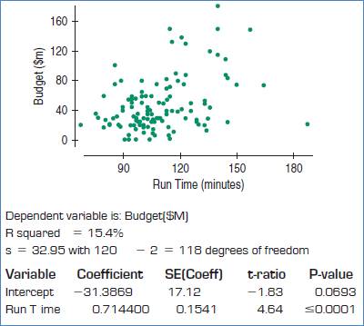
s = 32.95 is the standard deviation of the residuals.

Therefore, the actual values vary on average by 32.95 million dollars about the predicted values.

d)

To determine

To identify the values of the standard error of the slope of the regression line.

Answer to Problem 3E

SE_b = 0.1541

Explanation of Solution

Given:

  

  

The standard error of the slope of the regression line is,

SE_b = 0.1541 million dollars per minute of run time.

e)

To determine

To explain the value of the standard error of the slope of the regression line.

Explanation of Solution

Given:

  

  

The standard error of the slope of the regression line is,

SE_b = 0.1541 million dollars per minute of run time.

This means that the slope of the regression line of different samples is expected to vary on average by 0.1541 million dollars per minute of run time.