Draw a budget line.
Explanation of Solution
Budget constraint equation:
General budget constraint equation can be written as follows:
Substitute the respective values in Equation (1) to calculate the maximum quantity of Lat can buy (when the consumer buys 0 units of Sco) with initial price.
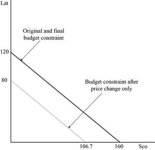
The maximum quantity of Lat is 120 units.
Substitute the respective values in equation (1) to calculate the maximum quantity of Sco can buy (when the consumer buys 0 units of Lat) with initial price.
The maximum quantity of Sco is 160 units.
Substitute the respective values in Equation (1) to calculate the maximum quantity of Lat can buy (when the consumer buys 0 units of Sco) with new price.
The maximum quantity of Lat is 80 units.
Substitute the respective values in Equation (1) to calculate the maximum quantity of Sco can buy (when the consumer buys 0 units of Lat) with new price.
The maximum quantity of Sco is 106.67units.
Figure 1 illustrates the budget line for the different price levels.

Figure 1
In Figure 1, the horizontal axis measures the quantity of Sco and the vertical axis measures the quantity of Lat. When the income is fixed, increasing price reduces the quantity of goods that can be purchased. This would shift the budget line inward.
Substitute the respective values in Equation (1) to calculate the maximum quantity of Lat can buy (when the consumer buys 0 units of Sco) with new price and new income.
The maximum quantity of Lat is 120 units.
Substitute the respective values in Equation (1) to calculate the maximum quantity of Sco can buy (when the consumer buys 0 units of Lat) with new price.
The maximum quantity of Sco is 160units.
Figure 2 illustrates the budget line for the different price levels.
In Figure 2, the horizontal axis measures the quantity of Sco and the vertical axis measures the quantity of Lat. When the income increases, the quantity of goods that can be purchased would increase. This shifts the budget line outward to the initial level. The impact of increasing price of 50% for both the goods offset by increasing the income by 50% .
Concept Introduction:
Budget line: Budget line (Budget constraint) refers to all the possible combinations of goods and services that can be purchased with the entire income, at a given price level.
Want to see more full solutions like this?
Chapter 25 Solutions
Modern Principles of Economics

- 2. What is the payoff from a long futures position where you are obligated to buy at the contract price? What is the payoff from a short futures position where you are obligated to sell at the contract price?? Draw the payoff diagram for each position. Payoff from Futures Contract F=$50.85 S1 Long $100 $95 $90 $85 $80 $75 $70 $65 $60 $55 $50.85 $50 $45 $40 $35 $30 $25 Shortarrow_forward3. Consider a call on the same underlier (Cisco). The strike is $50.85, which is the forward price. The owner of the call has the choice or option to buy at the strike. They get to see the market price S1 before they decide. We assume they are rational. What is the payoff from owning (also known as being long) the call? What is the payoff from selling (also known as being short) the call? Payoff from Call with Strike of k=$50.85 S1 Long $100 $95 $90 $85 $80 $75 $70 $65 $60 $55 $50.85 $50 $45 $40 $35 $30 $25 Shortarrow_forward4. Consider a put on the same underlier (Cisco). The strike is $50.85, which is the forward price. The owner of the call has the choice or option to buy at the strike. They get to see the market price S1 before they decide. We assume they are rational. What is the payoff from owning (also known as being long) the put? What is the payoff from selling (also known as being short) the put? Payoff from Put with Strike of k=$50.85 S1 Long $100 $95 $90 $85 $80 $75 $70 $65 $60 $55 $50.85 $50 $45 $40 $35 $30 $25 Shortarrow_forward
- The following table provides information on two technology companies, IBM and Cisco. Use the data to answer the following questions. Company IBM Cisco Systems Stock Price Dividend (trailing 12 months) $150.00 $50.00 $7.00 Dividend (next 12 months) $7.35 Dividend Growth 5.0% $2.00 $2.15 7.5% 1. You buy a futures contract instead of purchasing Cisco stock at $50. What is the one-year futures price, assuming the risk-free interest rate is 6%? Remember to adjust the futures price for the dividend of $2.15.arrow_forward5. Consider a one-year European-style call option on Cisco stock. The strike is $50.85, which is the forward price. The risk-free interest rate is 6%. Assume the stock price either doubles or halves each period. The price movement corresponds to u = 2 and d = ½ = 1/u. S1 = $100 Call payoff= SO = $50 S1 = $25 Call payoff= What is the call payoff for $1 = $100? What is the call payoff for S1 = $25?arrow_forwardMC The diagram shows a pharmaceutical firm's demand curve and marginal cost curve for a new heart medication for which the firm holds a 20-year patent on its production. Assume this pharmaceutical firm charges a single price for its drug. At its profit-maximizing level of output, it will generate a total profit represented by OA. areas J+K. B. areas F+I+H+G+J+K OC. areas E+F+I+H+G. D. - it is not possible to determine with the informatio OE. the sum of areas A through K. (...) Po P1 Price F P2 E H 0 G B Q MR D ōarrow_forward
- Price Quantity $26 0 The marketing department of $24 20,000 Johnny Rockabilly's record company $22 40,000 has determined that the demand for his $20 60,000 latest CD is given in the table at right. $18 80,000 $16 100,000 $14 120,000 The record company's costs consist of a $240,000 fixed cost of recording the CD, an $8 per CD variable cost of producing and distributing the CD, plus the cost of paying Johnny for his creative talent. The company is considering two plans for paying Johnny. Plan 1: Johnny receives a zero fixed recording fee and a $4 per CD royalty for each CD that is sold. Plan 2: Johnny receives a $400,000 fixed recording fee and zero royalty per CD sold. Under either plan, the record company will choose the price of Johnny's CD so as to maximize its (the record company's) profit. The record company's profit is the revenues minus costs, where the costs include the costs of production, distribution, and the payment made to Johnny. Johnny's payment will be be under plan 2 as…arrow_forwardWhich of the following is the best example of perfect price discrimination? A. Universities give entry scholarships to poorer students. B. Students pay lower prices at the local theatre. ○ C. A hotel charges for its rooms according to the number of days left before the check-in date. ○ D. People who collect the mail coupons get discounts at the local food store. ○ E. An airline offers a discount to students.arrow_forwardConsider the figure at the right. The profit of the single-price monopolist OA. is shown by area D+H+I+F+A. B. is shown by area A+I+F. OC. is shown by area D + H. ○ D. is zero. ○ E. cannot be calculated or shown with just the information given in the graph. (C) Price ($) B C D H FIG шо E MC ATC A MR D = AR Quantityarrow_forward
- Consider the figure. A perfectly price-discriminating monopolist will produce ○ A. 162 units and charge a price equal to $69. ○ B. 356 units and charge a price equal to $52 for the last unit sold only. OC. 162 units and charge a price equal to $52. OD. 356 units and charge a price equal to the perfectly competitive price. Dollars per Unit $69 $52 MR 162 356 Output MC Darrow_forwardThe figure at right shows the demand line, marginal revenue line, and cost curves for a single-price monopolist. Now suppose the monopolist is able to charge a different price on each different unit sold. The profit-maximizing quantity for the monopolist is (Round your response to the nearest whole number.) The price charged for the last unit sold by this monopolist is $ (Round your response to the nearest dollar.) Price ($) 250 225- 200- The monopolist's profit is $ the nearest dollar.) (Round your response to MC 175- 150 ATC 125- 100- 75- 50- 25- 0- °- 0 20 40 60 MR 80 100 120 140 160 180 200 Quantityarrow_forwardThe diagram shows a pharmaceutical firm's demand curve and marginal cost curve for a new heart medication for which the firm holds a 20-year patent on its production. At its profit-maximizing level of output, it will generate a deadweight loss to society represented by what? A. There is no deadweight loss generated. B. Area H+I+J+K OC. Area H+I D. Area D + E ◇ E. It is not possible to determine with the information provided. (...) 0 Price 0 m H B GI A MR MC D Outparrow_forward

 Principles of Economics (12th Edition)EconomicsISBN:9780134078779Author:Karl E. Case, Ray C. Fair, Sharon E. OsterPublisher:PEARSON
 Engineering Economy (17th Edition)EconomicsISBN:9780134870069Author:William G. Sullivan, Elin M. Wicks, C. Patrick KoellingPublisher:PEARSON
 Principles of Economics (MindTap Course List)EconomicsISBN:9781305585126Author:N. Gregory MankiwPublisher:Cengage Learning
 Managerial Economics: A Problem Solving ApproachEconomicsISBN:9781337106665Author:Luke M. Froeb, Brian T. McCann, Michael R. Ward, Mike ShorPublisher:Cengage Learning
 Managerial Economics & Business Strategy (Mcgraw-...EconomicsISBN:9781259290619Author:Michael Baye, Jeff PrincePublisher:McGraw-Hill Education