
a.
To construct: The 99% confidence interval for the proportion of Americans who are more than 18 years of age and using social networking sites on their phones.
a.
Answer to Problem 25.43E
The 99% confidence interval for the proportion of Americans who are more than 18 years of age and using social networking sites on their phones is 0.3039 to 0.3593 or 30.39% to 35.93%.
Explanation of Solution
Given info:
The data shows the number of cell phone users who tend to use social media on their phones and the data is separated according to their age group.
Calculation:
Let
Thus, the proportion of Americans who are more than 18 years of age and using social networking sites on their phones is 0.3316.
Software procedure:
Step-by-step procedure for constructing 99% confidence interval for the given proportion is shown below:
- Click on Stat, Basic statistics and 1-proportion.
- Choose Summarized data, under Number of
events enter636, under Number of trials enter 1,918. - Click on options, choose 99% confidence interval.
- Click ok.
Output using MINITAB is given below:
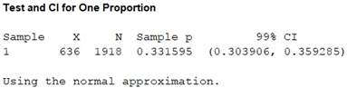
Thus, the 99% confidence interval for the proportion of Americans who are more than 18 years of age and using social networking sites on their phones is 0.3039 to 0.3593.
b.
To compare: The two conditional distributions and also the graph of conditional distributions.
To find: The conditional distribution of age for the Americans who use social networking sites and who don’t use social networking sites on their phones.
To construct: A suitable graph for the conditional distribution of age for the Americans who use social networking sites and who don’t use social networking sites on their phones.
b.
Answer to Problem 25.43E
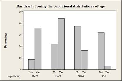
The Americans who are aged below 50 have ahigher percentage for using social networking sites on their phones, whereas Americans who are aged greater than 50 are using comparatively less percentage of social networking sites on their phones.
The conditional distribution of age for the Americans who use social networking sites and who don’t use social networking sites on their phones is given below:
| Age Group | Conditional distribution age for the Americans who use social networking sites and who don’t use social networking sites on their phones | |
| Yes | No | |
| 18-29 | 35.85 | 8.74 |
| 30-49 | 44.18 | 21.92 |
| 50-64 | 16.67 | 37.52 |
| 65+ | 3.30 | 31.83 |
The bar graph showing the conditional distribution of age for the Americans who use social networking sites and who don’t use social networking sites on their phones is given below:
Output obtained from MINITAB is given below:
Explanation of Solution
Calculation:
The conditional distribution of age for the Americans who use social networking sites on their phones is calculated as follows:
The conditional distribution of age for the Americans who don’t use social networking sites on their phones is calculated as follows:
The conditional distribution age for the Americans who use social networking sites and who don’t use social networking sites on their phones is given below:
| Conditional distribution age for the Americans who use social networking sites and who don’t use social networking sites on their phones | ||
| AgeGroup | Yes | No |
| 18-29 | ||
| 30-49 | ||
| 50-64 | ||
| 65+ | ||
Software Procedure:
Step-by-step procedure to construct the Bar Chart using the MINITAB software:
- Choose Graph > Bar Chart.
- From Bars represent, choose Values from a table.
- Under TwoColumns of values, choose Cluster. Click OK.
- In Graph variables, enter the columns of Yes and No.
- In Row labels, enter “Age Group”.
- In Table arrangement, click “Rows are outermost categories and columns are innermost”.
- Click OK.
Interpretation:
The bar chart for comparing two conditional distributions is constructed with bars to the extreme left side of the graph, which represents the age group 18-29. Similarly, the other age groups are shown.
Justification:
The bar graph and the conditional distributions show that Americans who are aged below 50 are using the social media network much more when compared to the age group 50-65 and 65+
c.
To test: Whether there is a significant difference in the distribution of age group on social network media usage.
To find: The mean value of the test statistic given that the null hypothesis is true.
To give: The P-value.
c.
Answer to Problem 25.43E
There is a significant difference in the distribution of age group on social network media usage.
The mean value of the chi-square test statistic given that the null hypothesis is true is given is to be 3.
The P-value is 0.000.
Explanation of Solution
Calculation:
The claim is to test whether there is any significant difference in the distribution of age group on social network media usage.
Cell frequency for using Chi-square test:
- When at most 20% of the cell frequencies are less than 5
- If all the individual frequencies are 1 or more than 1.
- All the expected frequencies must be 5 or greater than 5
The hypotheses used for testing are given below:
Software procedure:
Step-by-step procedure for calculating the chi-square test statistic is given below:
- Click on Stat, select Tables and then click on Chi-square Test (Two-way table in a worksheet).
- Under Columns containing the table: enter the columns of Yes and No.
- Click ok.
Output obtained from MINITAB is given below:
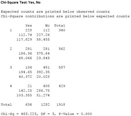
Thus, the test statistic is 463.223, the degree of freedom is 3, and the P-value is 0.000.
Since all the expected frequencies are greater than 5, the usage of chi-square test is appropriate.
Conclusion:
The P-value is 0.000 and the level of significance is 0.05.
Here, the P-value is less than the level of significance.
Therefore, the null hypothesis is rejected.
Thus, there is sufficient evidence to support the claim that there is a significant difference in the distribution of age groups on social network media usage.
Justification:
Fact:
If the null hypothesis is true, then the mean of any chi-square distribution is equal to its degrees of freedom.
From the MINITAB output, it can be observed that the degree of freedom is calculated as 3. So, the mean value of the chi-square statistic is 3.
Thus, the mean value of the chi-square statistic is 3.
Also, the observed chi-square value is
d.
To give: A comparison for the difference in the distribution of age across social media network usage.
d.
Answer to Problem 25.43E
The age group 18-29 who have said “Yes” and the 65+ age group who have said “Yes” are contributing more to the chi-square test statistic.
The comparison shows that the age group 18 and below 50 are using social network media on their phones in a higher percentage when compared with the other age group or other people.
Explanation of Solution
From the MINITAB output, it can be seen that the observed frequencies for age group 18-29, 30-49 are higher than the expected frequency, given that the null hypothesis is true.
The age group 65+ that observed frequency for “Yes” is less than the expected frequency, given that the null hypothesis is true.
Want to see more full solutions like this?
Chapter 25 Solutions
The Basic Practice of Statistics

- Please conduct a step by step of these statistical tests on separate sheets of Microsoft Excel. If the calculations in Microsoft Excel are incorrect, the null and alternative hypotheses, as well as the conclusions drawn from them, will be meaningless and will not receive any points. 4. One-Way ANOVA: Analyze the customer satisfaction scores across four different product categories to determine if there is a significant difference in means. (Hints: The null can be about maintaining status-quo or no difference among groups) H0 = H1=arrow_forwardPlease conduct a step by step of these statistical tests on separate sheets of Microsoft Excel. If the calculations in Microsoft Excel are incorrect, the null and alternative hypotheses, as well as the conclusions drawn from them, will be meaningless and will not receive any points 2. Two-Sample T-Test: Compare the average sales revenue of two different regions to determine if there is a significant difference. (Hints: The null can be about maintaining status-quo or no difference among groups; if alternative hypothesis is non-directional use the two-tailed p-value from excel file to make a decision about rejecting or not rejecting null) H0 = H1=arrow_forwardPlease conduct a step by step of these statistical tests on separate sheets of Microsoft Excel. If the calculations in Microsoft Excel are incorrect, the null and alternative hypotheses, as well as the conclusions drawn from them, will be meaningless and will not receive any points 3. Paired T-Test: A company implemented a training program to improve employee performance. To evaluate the effectiveness of the program, the company recorded the test scores of 25 employees before and after the training. Determine if the training program is effective in terms of scores of participants before and after the training. (Hints: The null can be about maintaining status-quo or no difference among groups; if alternative hypothesis is non-directional, use the two-tailed p-value from excel file to make a decision about rejecting or not rejecting the null) H0 = H1= Conclusion:arrow_forward
- Please conduct a step by step of these statistical tests on separate sheets of Microsoft Excel. If the calculations in Microsoft Excel are incorrect, the null and alternative hypotheses, as well as the conclusions drawn from them, will be meaningless and will not receive any points. The data for the following questions is provided in Microsoft Excel file on 4 separate sheets. Please conduct these statistical tests on separate sheets of Microsoft Excel. If the calculations in Microsoft Excel are incorrect, the null and alternative hypotheses, as well as the conclusions drawn from them, will be meaningless and will not receive any points. 1. One Sample T-Test: Determine whether the average satisfaction rating of customers for a product is significantly different from a hypothetical mean of 75. (Hints: The null can be about maintaining status-quo or no difference; If your alternative hypothesis is non-directional (e.g., μ≠75), you should use the two-tailed p-value from excel file to…arrow_forwardPlease conduct a step by step of these statistical tests on separate sheets of Microsoft Excel. If the calculations in Microsoft Excel are incorrect, the null and alternative hypotheses, as well as the conclusions drawn from them, will be meaningless and will not receive any points. 1. One Sample T-Test: Determine whether the average satisfaction rating of customers for a product is significantly different from a hypothetical mean of 75. (Hints: The null can be about maintaining status-quo or no difference; If your alternative hypothesis is non-directional (e.g., μ≠75), you should use the two-tailed p-value from excel file to make a decision about rejecting or not rejecting null. If alternative is directional (e.g., μ < 75), you should use the lower-tailed p-value. For alternative hypothesis μ > 75, you should use the upper-tailed p-value.) H0 = H1= Conclusion: The p value from one sample t-test is _______. Since the two-tailed p-value is _______ 2. Two-Sample T-Test:…arrow_forwardPlease conduct a step by step of these statistical tests on separate sheets of Microsoft Excel. If the calculations in Microsoft Excel are incorrect, the null and alternative hypotheses, as well as the conclusions drawn from them, will be meaningless and will not receive any points. What is one sample T-test? Give an example of business application of this test? What is Two-Sample T-Test. Give an example of business application of this test? .What is paired T-test. Give an example of business application of this test? What is one way ANOVA test. Give an example of business application of this test? 1. One Sample T-Test: Determine whether the average satisfaction rating of customers for a product is significantly different from a hypothetical mean of 75. (Hints: The null can be about maintaining status-quo or no difference; If your alternative hypothesis is non-directional (e.g., μ≠75), you should use the two-tailed p-value from excel file to make a decision about rejecting or not…arrow_forward
- The data for the following questions is provided in Microsoft Excel file on 4 separate sheets. Please conduct a step by step of these statistical tests on separate sheets of Microsoft Excel. If the calculations in Microsoft Excel are incorrect, the null and alternative hypotheses, as well as the conclusions drawn from them, will be meaningless and will not receive any points. What is one sample T-test? Give an example of business application of this test? What is Two-Sample T-Test. Give an example of business application of this test? .What is paired T-test. Give an example of business application of this test? What is one way ANOVA test. Give an example of business application of this test? 1. One Sample T-Test: Determine whether the average satisfaction rating of customers for a product is significantly different from a hypothetical mean of 75. (Hints: The null can be about maintaining status-quo or no difference; If your alternative hypothesis is non-directional (e.g., μ≠75), you…arrow_forwardWhat is one sample T-test? Give an example of business application of this test? What is Two-Sample T-Test. Give an example of business application of this test? .What is paired T-test. Give an example of business application of this test? What is one way ANOVA test. Give an example of business application of this test? 1. One Sample T-Test: Determine whether the average satisfaction rating of customers for a product is significantly different from a hypothetical mean of 75. (Hints: The null can be about maintaining status-quo or no difference; If your alternative hypothesis is non-directional (e.g., μ≠75), you should use the two-tailed p-value from excel file to make a decision about rejecting or not rejecting null. If alternative is directional (e.g., μ < 75), you should use the lower-tailed p-value. For alternative hypothesis μ > 75, you should use the upper-tailed p-value.) H0 = H1= Conclusion: The p value from one sample t-test is _______. Since the two-tailed p-value…arrow_forward4. Dynamic regression (adapted from Q10.4 in Hyndman & Athanasopoulos) This exercise concerns aus_accommodation: the total quarterly takings from accommodation and the room occupancy level for hotels, motels, and guest houses in Australia, between January 1998 and June 2016. Total quarterly takings are in millions of Australian dollars. a. Perform inflation adjustment for Takings (using the CPI column), creating a new column in the tsibble called Adj Takings. b. For each state, fit a dynamic regression model of Adj Takings with seasonal dummy variables, a piecewise linear time trend with one knot at 2008 Q1, and ARIMA errors. c. What model was fitted for the state of Victoria? Does the time series exhibit constant seasonality? d. Check that the residuals of the model in c) look like white noise.arrow_forward
- ce- 216 Answer the following, using the figures and tables from the age versus bone loss data in 2010 Questions 2 and 12: a. For what ages is it reasonable to use the regression line to predict bone loss? b. Interpret the slope in the context of this wolf X problem. y min ball bas oft c. Using the data from the study, can you say that age causes bone loss? srls to sqota bri vo X 1931s aqsini-Y ST.0 0 Isups Iq nsalst ever tom vam noboslios tsb a ti segood insvla villemari aixs-Yediarrow_forward120 110 110 100 90 80 Total Score Scatterplot of Total Score vs. Putts grit bas 70- 20 25 30 35 40 45 50 Puttsarrow_forward10 15 Answer the following, using the figures and tables from the temperature versus coffee sales data from Questions 1 and 11: a. How many coffees should the manager prepare to make if the temperature is 32°F? b. As the temperature drops, how much more coffee will consumers purchase?ov (Hint: Use the slope.) 21 bru sug c. For what temperature values does the voy marw regression line make the best predictions? al X al 1090391-Yrit,vewolf 30-X Inlog arts bauoxs 268 PART 4 Statistical Studies and the Hunt forarrow_forward
 MATLAB: An Introduction with ApplicationsStatisticsISBN:9781119256830Author:Amos GilatPublisher:John Wiley & Sons Inc
 Probability and Statistics for Engineering and th...StatisticsISBN:9781305251809Author:Jay L. DevorePublisher:Cengage Learning
 Statistics for The Behavioral Sciences (MindTap C...StatisticsISBN:9781305504912Author:Frederick J Gravetter, Larry B. WallnauPublisher:Cengage Learning
 Elementary Statistics: Picturing the World (7th E...StatisticsISBN:9780134683416Author:Ron Larson, Betsy FarberPublisher:PEARSON
 The Basic Practice of StatisticsStatisticsISBN:9781319042578Author:David S. Moore, William I. Notz, Michael A. FlignerPublisher:W. H. Freeman
 Introduction to the Practice of StatisticsStatisticsISBN:9781319013387Author:David S. Moore, George P. McCabe, Bruce A. CraigPublisher:W. H. Freeman