
a.
To construct: The 99% confidence interval for the proportion of Americans who are more than 50 years of age and also current smokers.
a.
Answer to Problem 25.42E
The 99% confidence interval for the proportion of Americans who are more than 50 years of age and also current smokers is 0.0826 to 0.1057or 8.26% to 10.57%.
Explanation of Solution
Given info:
The data shows the results obtained by asking two questions to a random sample of 50 year old adults “How do your overall health, excellent, very good, good, fair and poor?” and the second question is “Do you smoke currently, yes or no?”
Calculation:
Let
Thus, the proportion of Americans who are more than 50 years of age and currently smoking is 0.094.
Software procedure:
Step-by-step procedure for constructing 99% confidence interval for the given proportion is shown below:
- Click on Stat, Basic statistics and 1-proportion.
- Choose Summarized data, under Number of
events enter 404, under Number of trials enter 4,310. - Click on options, choose 99% confidence interval.
- Click ok.
Output using MINITAB is given below:
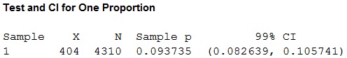
Thus, the 99% confidence interval for the proportion of Americans who are more than who are more than 50 years of age and also current smokers is 0.0826 to 0.1057.
b.
To compare: The two conditional distributions and also the graph of conditional distributions.
To find: The conditional distribution of age for the Americans who use social networking sitesand who don’t use social networking siteson their phones.
To construct: A suitable graph for the conditional distribution of age for the Americans who use social networking sitesand who don’t use social networking siteson their phones.
b.
Answer to Problem 25.42E
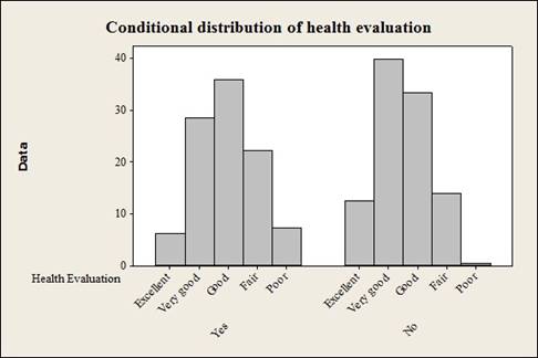
- The bar graph and the conditional distributions show that Americans are currently smoking have lowest percentages in “excellent” and “very good” health evaluation whereas Americans who are not currently smoking have highest percentages in “excellent” and “very good” health evaluation.
- The percentages in “fair and poor” health evaluation is more in currently smoking group when compared to the percentages for the same categories under not currently smoking group.
The conditional distribution of health evaluation for the Americans who are currently smoking and not currently smoking is given below:
|
Conditional distribution of health evaluation for the Americans who are currently smoking and not currently smoking | ||
| Health Evaluation | Yes | No |
| Excellent | 6.20 | 12.4 |
| Very good | 28.50 | 39.9 |
| Good | 35.90 | 33.5 |
| Fair | 22.30 | 14.0 |
| Poor | 7.18 | 0.3 |
The bar graph showing the conditional distribution of health evaluation for the Americans who are currently smoking and not currently smoking is given below:
- Output obtained from MINITAB is given below:
Explanation of Solution
Calculation:
The conditional distribution of health evaluation for the Americans who are current smokers is calculated as follows:
The conditional distribution of health evaluation for the Americans who are not current smokers is calculated as follows:
The conditional distribution of health evaluation for the Americans who are currently smoking and not currently smoking is given below:
| Conditional distribution of health evaluation for the Americans who are currently smoking and not currently smoking | ||
| Health Evaluation | Yes | No |
| Excellent |
|
|
| Very good |
|
|
| Good |
|
|
| Fair |
|
|
| Poor |
|
|
Software Procedure:
Step-by-step procedure to construct the Bar Chart using the MINITAB software:
- Choose Graph > Bar Chart.
- From Bars represent, choose Values from a table.
- Under Two Columns of values, choose Cluster. Click OK.
- In Graph variables, enter the columns of Yes and No.
- In Row labels, enter “Health Evaluation”.
- In Table arrangement, click “columns are outermost categories and columns are innermost”.
- Click OK.
- Interpretation:
- The bar chart for comparing two conditional distributions is constructed with bars to the extreme left side of the graph, which represents the currently smoking group.
- c.
- To test: Whether there is a significant difference between health evaluation and currently smoking and not currently smoking group.
- To find: The mean value of the test statistic given that the null hypothesis is true.
- To give: The P-value.
- c.
Answer to Problem 25.42E
- There is a significant difference between health evaluation and currently smoking and not currently smoking group.
- The mean value of the chi-square test statistic given that the null hypothesis is true is given is to be 4.
- The P-value is 0.000.
Explanation of Solution
- Calculation:
- The claim is to test whether there is any significant difference between health evaluation and currently smoking and not currently smoking group.
Cell frequency for using Chi-square test:
- When at most 20% of the cell frequencies are less than 5
- If all the individual frequencies are 1 or more than 1.
- All the expected frequencies must be 5 or greater than 5
The hypotheses used for testing are given below:
Software procedure:
Step-by-stepprocedure for calculating the chi-square test statistic is given below:
- Click on Stat, select Tables and then click on Chi-square Test (Two-way table in a worksheet).
- Under Columns containing the table: enter the columns of Yes and No.
- Click ok.
Output obtained from MINITAB is given below:
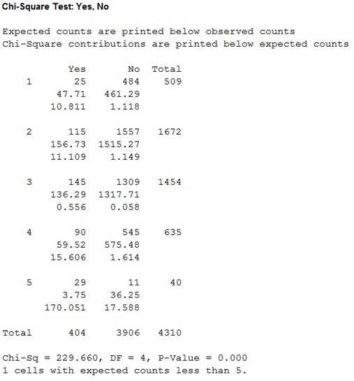
Thus, the test statistic is 229.660, the degree of freedom is 4, and the P-value is 0.000.
Only one cell is having an expected frequency less than 5. The usage of chi-square test is appropriate.
Conclusion:
The P-value is 0.000 and the level of significance is 0.05.
Here, the P-value is less than the level of significance.
Therefore, the null hypothesis is rejected.
Thus, there is sufficient evidence to support the claim that there is a significant difference between health evaluation and currently smoking and not currently smoking group.
Justification:
Fact:
If the null hypothesis is true, then the mean of any chi-square distribution is equal to its degrees of freedom.
From the MINITAB output, it can be observed that the degree of freedom is calculated as 3. So, the mean value of the chi-square statistic is 3.
Thus, the mean value of the chi-square statistic is 3.
Also, the observed chi-square value is
d.
To give: A comparison for the difference in the distribution of age across social media network usage.
d.
Explanation of Solution
Comparison:
From the MINITAB output, it can be seen that the observed frequencies for good, fair and poor health evaluation for currently smoking group is higher than the expected frequency, given that the null hypothesis is true.
In non-smoking group the observed frequencies for good, fair and poor health evaluation is lesser than the expected frequency.
The people who are currently smoking have a poor health condition when compared to the non smoking group.
Hence, there is a significant difference in the health evaluation for currently smoking and not currently smoking group.
Want to see more full solutions like this?
Chapter 25 Solutions
EBK THE BASIC PRACTICE OF STATISTICS

- For a binary asymmetric channel with Py|X(0|1) = 0.1 and Py|X(1|0) = 0.2; PX(0) = 0.4 isthe probability of a bit of “0” being transmitted. X is the transmitted digit, and Y is the received digit.a. Find the values of Py(0) and Py(1).b. What is the probability that only 0s will be received for a sequence of 10 digits transmitted?c. What is the probability that 8 1s and 2 0s will be received for the same sequence of 10 digits?d. What is the probability that at least 5 0s will be received for the same sequence of 10 digits?arrow_forwardV2 360 Step down + I₁ = I2 10KVA 120V 10KVA 1₂ = 360-120 or 2nd Ratio's V₂ m 120 Ratio= 360 √2 H I2 I, + I2 120arrow_forwardQ2. [20 points] An amplitude X of a Gaussian signal x(t) has a mean value of 2 and an RMS value of √(10), i.e. square root of 10. Determine the PDF of x(t).arrow_forward
- In a network with 12 links, one of the links has failed. The failed link is randomlylocated. An electrical engineer tests the links one by one until the failed link is found.a. What is the probability that the engineer will find the failed link in the first test?b. What is the probability that the engineer will find the failed link in five tests?Note: You should assume that for Part b, the five tests are done consecutively.arrow_forwardProblem 3. Pricing a multi-stock option the Margrabe formula The purpose of this problem is to price a swap option in a 2-stock model, similarly as what we did in the example in the lectures. We consider a two-dimensional Brownian motion given by W₁ = (W(¹), W(2)) on a probability space (Q, F,P). Two stock prices are modeled by the following equations: dX = dY₁ = X₁ (rdt+ rdt+0₁dW!) (²)), Y₁ (rdt+dW+0zdW!"), with Xo xo and Yo =yo. This corresponds to the multi-stock model studied in class, but with notation (X+, Y₁) instead of (S(1), S(2)). Given the model above, the measure P is already the risk-neutral measure (Both stocks have rate of return r). We write σ = 0₁+0%. We consider a swap option, which gives you the right, at time T, to exchange one share of X for one share of Y. That is, the option has payoff F=(Yr-XT). (a) We first assume that r = 0 (for questions (a)-(f)). Write an explicit expression for the process Xt. Reminder before proceeding to question (b): Girsanov's theorem…arrow_forwardProblem 1. Multi-stock model We consider a 2-stock model similar to the one studied in class. Namely, we consider = S(1) S(2) = S(¹) exp (σ1B(1) + (M1 - 0/1 ) S(²) exp (02B(2) + (H₂- M2 where (B(¹) ) +20 and (B(2) ) +≥o are two Brownian motions, with t≥0 Cov (B(¹), B(2)) = p min{t, s}. " The purpose of this problem is to prove that there indeed exists a 2-dimensional Brownian motion (W+)+20 (W(1), W(2))+20 such that = S(1) S(2) = = S(¹) exp (011W(¹) + (μ₁ - 01/1) t) 롱) S(²) exp (021W (1) + 022W(2) + (112 - 03/01/12) t). where σ11, 21, 22 are constants to be determined (as functions of σ1, σ2, p). Hint: The constants will follow the formulas developed in the lectures. (a) To show existence of (Ŵ+), first write the expression for both W. (¹) and W (2) functions of (B(1), B(²)). as (b) Using the formulas obtained in (a), show that the process (WA) is actually a 2- dimensional standard Brownian motion (i.e. show that each component is normal, with mean 0, variance t, and that their…arrow_forward
- The scores of 8 students on the midterm exam and final exam were as follows. Student Midterm Final Anderson 98 89 Bailey 88 74 Cruz 87 97 DeSana 85 79 Erickson 85 94 Francis 83 71 Gray 74 98 Harris 70 91 Find the value of the (Spearman's) rank correlation coefficient test statistic that would be used to test the claim of no correlation between midterm score and final exam score. Round your answer to 3 places after the decimal point, if necessary. Test statistic: rs =arrow_forwardBusiness discussarrow_forwardBusiness discussarrow_forward
 MATLAB: An Introduction with ApplicationsStatisticsISBN:9781119256830Author:Amos GilatPublisher:John Wiley & Sons Inc
 Probability and Statistics for Engineering and th...StatisticsISBN:9781305251809Author:Jay L. DevorePublisher:Cengage Learning
 Statistics for The Behavioral Sciences (MindTap C...StatisticsISBN:9781305504912Author:Frederick J Gravetter, Larry B. WallnauPublisher:Cengage Learning
 Elementary Statistics: Picturing the World (7th E...StatisticsISBN:9780134683416Author:Ron Larson, Betsy FarberPublisher:PEARSON
 The Basic Practice of StatisticsStatisticsISBN:9781319042578Author:David S. Moore, William I. Notz, Michael A. FlignerPublisher:W. H. Freeman
 Introduction to the Practice of StatisticsStatisticsISBN:9781319013387Author:David S. Moore, George P. McCabe, Bruce A. CraigPublisher:W. H. Freeman