
To find: The 95% confidence interval for the
Answer to Problem 24.1TY
Option (c): (111.2, 118.6).
Explanation of Solution
Reason for the correct option:
Software procedure:
Step by step procedure to obtain the confidence interval using the MINITAB software:
- Choose Stat > Basic Statistics > 1-Sample t.
- In Summarized data, enter the
sample size as 27 and mean as 114.9. - In Standard deviation, enter the value as 9.3.
- Check Options, enter Confidence level as 95.0.
- Choose not equal in alternative.
- Click OK in all dialogue boxes.
Output using the MINITAB software is given below:
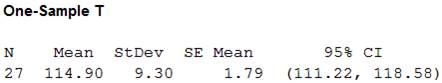
Thus, the 95% confidence interval for the mean blood pressure in the population from which the subjects were recruited is (111.2, 118.6).
Reason for the incorrect answer:
Option (a), Option (b) and Option (d) are incorrect, because the corresponding confidence intervals cannot be obtained from the formula of the confidence interval for the one-sample t procedures.
Therefore, the correct option is (b).
Introduction:
The formula for the confidence interval is,
Where,
Want to see more full solutions like this?
Chapter 24 Solutions
BASIC PRACTICE OF STATISTICS(REISSUE)>C

- Please help me with the following statistics problem A long-distance runner wants to compare the durability of two running shoe brands: Brand A and Brand B. Instead of testing them separately, 15 runners simultaneously wear Brand A on the left foot and Brand B on the right foot during training runs. The runner continues training as usual and tracks how many kilometers each shoe lasts before showing significant wear (e.g., loss of cushioning, outsole damage). Since both shoes experience the same runner, terrain, and conditions, any lifespan difference can be attributed to the shoe brand rather than external factors. Test whether Brand A running shoes have a significantly shorter lifespan than Brand B when worn under the same conditions by the same runner. CSV: "","A","B" "A",197,193 "B",230,229 "C",179,180 "D",206,205 "E",182,180 "F",141,142 "G",207,207 "H",116,112 "I",78,79 "J",0,0 "K",213,212 "L",86,83 "M",181,181 "N",85,79 "O",73,71 The…arrow_forwardAn article appeared in the Journal of Gambling Issues, in which the authors looked at random samples of Ontario residents who (i) have not completed some form of post-secondary education and (ii) have completed some form of post-secondary education. A code of 0 indicates the person does not have a gambling problem, a code of 1 indicates the person does have a gambling problem. The data is found in the accompanying data file. Download.csv file To count the frequencies of 0 and 1 in each sample, use the table(your_dataset_name$ column's name) function. Make sure to replace "your_dataset_name" with the actual name of your data file and specify the correct column name. For example: table(file60c5d1286c735$ CompletedPSEducation) Let PNOPS represent the proportion of persons not completing some form of post-secondary education who have a gambling problem, and PPs be the proportion of persons having completed post-secondary education who have a gambling problem. (a) Find a 92% confidence…arrow_forwardWe consider a (European) call option on a stock with expiration in 3 months and strike price $10. The annual interest rate on the market is r = 4%. The current price of the stock is $10 and we assume that the stock follows a geometric Brownian motion (Black-Scholes) model with parameters = 6% and σ = 0.2. (a) Determine the price Fo of this option at time t = : 0 (today). (b) Using the formulas provided in the lecture videos, calculate the value of each of the Greeks for this option. Namely, calculate A, T, v, О, p. (c) Find a formula for the change of the option price with respect to a change in the af (St, t) Әк strike price. In other words, determine (d) For each of the suggested modifications below, use an approximation to determine the change in the price of the option above without actually recalculating the price. For each one, provide an intuitive argument to explain why the price increases or decreases. (i) The rate of return μ decreases to 5%. (ii) The interest rate r…arrow_forward
- A box containing 24 seemly identical resistors has just been received. However,unbeknownst, 4 of these resistors are defective. a. Five resistors are randomly selected from this box without replacement (oncemoved from the box it is not returned to the box), what is the probability that oneor more of the defective resistors is among those selected? b. Five resistors are randomly selected from this box with replacement (after theresistor is removed and checked, it is returned to the box prior to the nextselection (hence the same resistor can be selected more than once)), what is theprobability that one or more of the defective resistors is among those selected?arrow_forwardBusiness Discussarrow_forwardTriola statistics Readers who prefer printed books Readers who prefer e-booksarrow_forward
- The following is a list of data on the duration of a sample of 200 outbreaks, in hours. 107 73 68 97 76 79 94 59 98 57 54 65 71 70 84 88 62 82 61 79 98 66 62 79 86 68 74 61 62 116 65 88 64 79 78 74 92 75 5289 85 28 73 80 68 78 89 72 78 88 77 103 88 63 68 90 62 89 71 71 74 222 R 82 79 70 ST☑ 65 98 77 86 58 69 88 81 74 70 65 81 75 81 78 90 78 96 75 KRRE F S 62 94 62 79 83 93 135 71 85 84 83 63 61 65 83 70 70 81 77 72 84 33 62 92 65 67 59 58 66 66 94 77 63 71 101 78 43 78 66 75 68 76 59 67 61 71 64 76 72 77 74 65 82 86 66 86 68 85 27% 96 72 77 60 67 87 83 68 72 74 91 76 83 งงง 8 སྐྱ ཐྭ ༄ ཏྱཾ 89 81 71 85 99 59 92 87 84 75 77 51 45 80 84 93 69 76 89 75 67 92 89 82 96 77 102 66 68 61 73 72 76 73 77 79 94 63 59 62 71 81 65 73 63 63 89 82 64 85 92 64 73 a. What is the variable? What type? b. Construct an interval-frequency table, with columns containing: class mark, absolute frequency, relative frequency, cumulative frequency, cumulative relative frequency, and percentage frequency.arrow_forwardThis is the information about the actors who won the Best Actor Oscar: Best actors 44 41 62 52 41 34 34 52 41 37 38 34 32 40 43 56 41 39 49 57 35 30 39 41 44 41 38 42 52 51 49 35 47 31 47 37 57 42 45 42 44 62 43 42 48 49 56 38 60 30 40 42 36 76 39 53 45 36 62 43 51 32 42 54 52 37 38 32 45 60 46 40 36 47 29 43 a. What is the variable? What type? b. Construct an interval-frequency table, with columns containing: class mark, absolute frequency, relative frequency, cumulative frequency, cumulative relative frequency, and percentage frequency.arrow_forwardans c plsarrow_forward
- Critically analyze the following graph and, based on statistical information, indicate the type of error it presents IN NO MORE THAN 3 LINES SCOTCEN POLL OF POLLS SHOULD SCOTLAND BE INDEPENDENT? NO 52% YES 58% LIVE CAW NAS & 28.30 HAS KILLED MORE THAN 2,600 IN WEST AFRICA, WORLD HEALTH ORG. BROOKEBCNNarrow_forwardCritically analyze the following graph and, based on statistical information, indicate the type of error it presents IN NO MORE THAN 3 LINES PRESIDENTIAL PREFERENCES RODOLFO CARTER 3% (+2pts) EVELYN MATTHEI 22% (+6pts) With the exception of President Boric, could you tell me who you would like to be the next president of Chile? CAMILA VALLEJO 4% (+2pts) JOSÉ ANTONIO KAST 19% (+5pts) MICHELLE BACHELET 6% (+1pts)arrow_forwardCritically analyze the following graph and, based on statistical information, indicate the type of error it presents IN NO MORE THAN 3 LINES 13% APPROVE 4% DOESN'T KNOW DOESN'T RESPOND 5% NEITHER APPROVES NOR DISAPPROVES 78% DISAPPROVES SURVEY PRESIDENTIAL APPROVAL DROPS TO 13%arrow_forward
 MATLAB: An Introduction with ApplicationsStatisticsISBN:9781119256830Author:Amos GilatPublisher:John Wiley & Sons Inc
 Probability and Statistics for Engineering and th...StatisticsISBN:9781305251809Author:Jay L. DevorePublisher:Cengage Learning
 Statistics for The Behavioral Sciences (MindTap C...StatisticsISBN:9781305504912Author:Frederick J Gravetter, Larry B. WallnauPublisher:Cengage Learning
 Elementary Statistics: Picturing the World (7th E...StatisticsISBN:9780134683416Author:Ron Larson, Betsy FarberPublisher:PEARSON
 The Basic Practice of StatisticsStatisticsISBN:9781319042578Author:David S. Moore, William I. Notz, Michael A. FlignerPublisher:W. H. Freeman
 Introduction to the Practice of StatisticsStatisticsISBN:9781319013387Author:David S. Moore, George P. McCabe, Bruce A. CraigPublisher:W. H. Freeman