
ESSENTIALS OF STATISTICS 6TH ED W/MYSTA
6th Edition
ISBN: 9781323845820
Author: Triola
Publisher: PEARSON
expand_more
expand_more
format_list_bulleted
Videos
Textbook Question
Chapter 2.3, Problem 9BSC
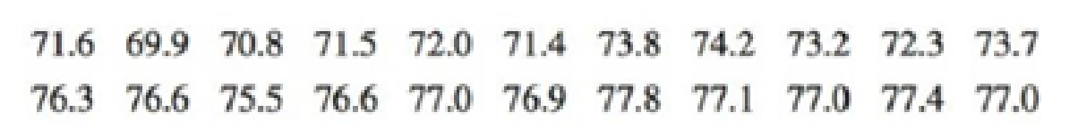
Time-Series Graphs. In Exercises 9 and 10, construct the time-series graph.
9. Gender Pay Gap Listed below are women’s
Expert Solution & Answer
Want to see the full answer?
Check out a sample textbook solution
Students have asked these similar questions
Write a Regression summary explaining significance of mode, explaining regression coefficients, significance of the independent variables, R and R square.
Premiums earned
Net income
Dividends
Underwriting Gain/ Loss
30.2
1.6
0.6
0.1
47.2
0.6
0.7
-3.6
92.8
8.4
1.8
-1.5
95.4
7.6
2
-4
100.4
6.3
2.2
-8.1
104.9
6.3
2.4
-10.8
113.2
2.2
2.3
-18.2
130.3
3.0
2.4
-21.4
161.9
13.5
2.3
-12.8
182.5
14.9
2.9
-5.9
193.3
11.7
2.9
-7.6
1- Let A = {A1, A2, ...), in which A, A, = 0, when i j.
a) Is A a π-system? If not, which element(s) should be added to A to become a π-system?
b) Prove that σ(A) consists of the finite or countable unions of elements of A; i.c., A E σ(A) if and
only if there exists finite or countable sequence {n} such that A = U₁An (Hint: Let F be such
class; prove that F is a σ-filed containing A.)
c) Let p ≥ 0 be a sequence of non-negative real numbers with Σip₁ = 1. Using p₁'s, how do you
construct a probability measure on σ(A)? (Hint: use extension theorem.)
2- Construct an example for which P(lim sup A,) = 1 and P(lim inf An) = 0.
In a town with 5000 adults, a sample of 50 is selected using SRSWOR and asked their opinion of a proposed municipal project; 30 are found to favor it and 20 oppose it. If, in fact, the adults of the town were equally divided on the proposal, what would be the probability of observing what has been observed? Approximate using the Binomial distribution. Compare this with the exact probability which is 0.0418.
Chapter 2 Solutions
ESSENTIALS OF STATISTICS 6TH ED W/MYSTA
Ch. 2.1 - McDonalds Dinner Service Times Refer 10 the...Ch. 2.1 - McDonalds Dinner Service Times Refer to the...Ch. 2.1 - Relative Frequency Distribution Use percentages to...Ch. 2.1 - Whats Wrong? Heights of adult males are known to...Ch. 2.1 - In Exercise 58, identify the class width, class...Ch. 2.1 - In Exercises 58, identify the class width, class...Ch. 2.1 - In Exercises 58, identify the class width, class...Ch. 2.1 - In Exercises 58, identify the class width, class...Ch. 2.1 - Normal Distributions. In Exercises 9 and 10, using...Ch. 2.1 - Normal Distributions. In Exercises 9 and 10, using...
Ch. 2.1 - Constructing Frequency Distributions. In Exercises...Ch. 2.1 - Constructing Frequency Distributions. In Exercises...Ch. 2.1 - Constructing Frequency Distributions. In Exercises...Ch. 2.1 - Burger King Dinner Service Times Refer to Data Set...Ch. 2.1 - Wendys Lunch Service Times Refer to Data Set 25...Ch. 2.1 - Wendys Dinner Service Times Refer to Data Set 25...Ch. 2.1 - Analysis of Last Digits Heights of statistics...Ch. 2.1 - Analysis of Last Digits Weights of respondents...Ch. 2.1 - Oscar Winners Construct one table (similar to...Ch. 2.1 - Blood Platelet Counts Construct one table (similar...Ch. 2.1 - Cumulative Frequency Distributions. In Exercises...Ch. 2.1 - Cumulative Frequency Distributions. In Exercises...Ch. 2.1 - Categorical Data. In Exercises 23 and 24, use the...Ch. 2.1 - Categorical Data. In Exercises 23 and 24, use the...Ch. 2.2 - Heights Heights of adult males are normally...Ch. 2.2 - More Heights The population of heights of adult...Ch. 2.2 - Blood Platelet Counts Listed below are blood...Ch. 2.2 - Blood Platelet Counts If we collect a sample of...Ch. 2.2 - Interpreting a Histogram. In Exercises 58, answer...Ch. 2.2 - Prob. 6BSCCh. 2.2 - Interpreting a Histogram. In Exercises 58, answer...Ch. 2.2 - Prob. 8BSCCh. 2.2 - Constructing Histograms. In Exercises 9-16,...Ch. 2.2 - Constructing Histograms. In Exercises 9-16,...Ch. 2.2 - Burger King Lunch Service Times Use the frequency...Ch. 2.2 - Burger King Dinner Service Times Use the frequency...Ch. 2.2 - Wendys Lunch Service Times Use the frequency...Ch. 2.2 - Wendys Dinner Service Times Use the frequency...Ch. 2.2 - Analysis of Last Digits Use the frequency...Ch. 2.2 - Analysis of Last Digits Use the frequency...Ch. 2.2 - Back-to-Back Relative Frequency Histograms When...Ch. 2.2 - Interpreting Normal Quantile Plots Which of the...Ch. 2.3 - Body Temperatures Listed below are body...Ch. 2.3 - Voluntary Response Data If we have a large...Ch. 2.3 - Ethics There are data showing that smoking is...Ch. 2.3 - CVDOT Section 2-1 introduced important...Ch. 2.3 - Dotplots. In Exercises 5 and 6, construct the...Ch. 2.3 - Diastolic Blood Pressure Listed below are...Ch. 2.3 - Stem plots. In Exercises 7 and 8, construct the...Ch. 2.3 - Stemplots. In Exercises 7 and 8, construct the...Ch. 2.3 - Time-Series Graphs. In Exercises 9 and 10,...Ch. 2.3 - Time-Series Graphs. In Exercises 9 and 10,...Ch. 2.3 - Pareto Charts. In Exercises 11 and 12 construct...Ch. 2.3 - Pareto Charts. In Exercises 11 and 12 construct...Ch. 2.3 - Pie Charts. In Exercises 13 and 14, construct the...Ch. 2.3 - Pie Charts. In Exercises 13 and 14, construct the...Ch. 2.3 - Frequency Polygon. In Exercises 15 and 16,...Ch. 2.3 - Frequency Polygon. In Exercises 15 and 16,...Ch. 2.3 - Self-Driving Vehicles In a survey of adults,...Ch. 2.3 - Deceptive Graphs. In Exercises 17-20, identify how...Ch. 2.3 - Deceptive Graphs. In Exercises 17-20, identify how...Ch. 2.3 - Deceptive Graphs. In Exercises 17-20, identify how...Ch. 2.3 - Expanded Stemplots A stemplot can be condensed by...Ch. 2.4 - Linear Correlation In this section we use r to...Ch. 2.4 - Causation A study has shown that there is a...Ch. 2.4 - Scanerplot What is a scatterplot and how does it...Ch. 2.4 - Estimating r For each of the following, estimate...Ch. 2.4 - Scatterplot. In Exercises 5-8, use the sample data...Ch. 2.4 - Scatterplot. In Exercises 5-8, use the sample data...Ch. 2.4 - Scatterplot. In Exercises 5-8, use the sample data...Ch. 2.4 - Scatterplot. In Exercises 5-8, use the sample data...Ch. 2.4 - Linear Correlation Coefficient In Exercises 9-12,...Ch. 2.4 - Linear Correlation Coefficient In Exercises 9-12,...Ch. 2.4 - Linear Correlation Coefficient In Exercises 9-12,...Ch. 2.4 - Using the data from Exercise 8 Heights of Fathers...Ch. 2.4 - Prob. 13BBCh. 2.4 - P-Values In Exercises 13-16, write a statement...Ch. 2.4 - P-Values In Exercises 13-16, write a statement...Ch. 2.4 - P-Values In Exercises 13-16, write a statement...Ch. 2 - Cookies Refer to the accompanying frequency...Ch. 2 - Cookies Using the same frequency distribution from...Ch. 2 - Cookies Using the same frequency distribution from...Ch. 2 - Cookies A stemplot of the same cookies summarized...Ch. 2 - Computers As a quality control manager at Texas...Ch. 2 - Distribution of Wealth In recent years, there has...Ch. 2 - Health Test In an investigation of a relationship...Ch. 2 - Lottery In Floridas Play 4 lottery game, four...Ch. 2 - Seatbelts The Beams Seatbelts company...Ch. 2 - Seatbelts A histogram is to be constructed from...Ch. 2 - Frequency Distribution of Body Temperatures...Ch. 2 - Histogram of Body Temperatures Construct the...Ch. 2 - Dotplot of Body Temperatures Construct a dotplot...Ch. 2 - Stemplot of Body Temperatures Construct a stemplot...Ch. 2 - Body Temperatures Listed below are the...Ch. 2 - Environment a. After collecting the average (mean)...Ch. 2 - Its Like Time Do This Exercise In a Marist survey...Ch. 2 - Whatever Use the same data from Exercise 7 to...Ch. 2 - In Exercises 1-6 refer to the data below, which...Ch. 2 - Frequency Distribution For the frequency...Ch. 2 - In Exercises 1-6, refer to the data below, which...Ch. 2 - In Exercises 1-6, refer to the data below, which...Ch. 2 - In Exercises 1-6, refer to the data below, which...Ch. 2 - Data Type a. The listed playing times are all...
Additional Math Textbook Solutions
Find more solutions based on key concepts
Determine the number of vectors , such that each is either 0 or 1 and
A First Course in Probability (10th Edition)
69. Get Started Early! Mitch and Bill are both age 75. When Mitch was 25 years old, he began depositing $1000 p...
Using and Understanding Mathematics: A Quantitative Reasoning Approach (6th Edition)
CHECK POINT 1 Find a counterexample to show that the statement The product of two two-digit numbers is a three-...
Thinking Mathematically (6th Edition)
To calculate the area of the trapezoid.
Pre-Algebra Student Edition
Stating the Null and Alternative Hypotheses In Exercises 25–30, write the claim as a mathematical statement. St...
Elementary Statistics: Picturing the World (7th Edition)
Knowledge Booster


Learn more about
Need a deep-dive on the concept behind this application? Look no further. Learn more about this topic, statistics and related others by exploring similar questions and additional content below.Similar questions
- Good explanation it sure experts solve itarrow_forwardBest explains it not need guidelines okkarrow_forwardActiv Determine compass error using amplitude (Sun). Minimum number of times that activity should be performed: 3 (1 each phase) Sample calculation (Amplitude- Sun): On 07th May 2006 at Sunset, a vessel in position 10°00'N 010°00'W observed the Sun bearing 288° by compass. Find the compass error. LMT Sunset: LIT: (+) 00d 07d 18h 00h 13m 40m UTC Sunset: 07d 18h 53m (added- since longitude is westerly) Declination (07d 18h): N 016° 55.5' d (0.7): (+) 00.6' Declination Sun: N 016° 56.1' Sin Amplitude = Sin Declination/Cos Latitude = Sin 016°56.1'/ Cos 10°00' = 0.295780189 Amplitude=W17.2N (The prefix of amplitude is named easterly if body is rising, and westerly if body is setting. The suffix is named same as declination) True Bearing=287.2° Compass Bearing= 288.0° Compass Error = 0.8° Westarrow_forward
- Only sure experts solve it correct complete solutions okkarrow_forward13. In 2000, two organizations conducted surveys to ascertain the public's opinion on banning gay men from serving in leadership roles in the Boy Scouts.• A Pew poll asked respondents whether they agreed with "the recent decision by the Supreme Court" that "the Boy Scouts of America have a constitutional right to block gay men from becoming troop leaders."A Los Angeles Times poll asked respondents whether they agreed with the following statement: "A Boy Scout leader should be removed from his duties as a troop leader if he is found out to be gay, even if he is considered by the Scout organization to be a model Boy Scout leader."One of these polls found 36% agreement; the other found 56% agreement. Which of the following statements is true?A) The Pew poll found 36% agreement, and the Los Angeles Times poll found 56% agreement.B) The Pew poll includes a leading question, while the Los Angeles Times poll uses neutral wording.C) The Los Angeles Times Poll includes a leading question, while…arrow_forwardAnswer questions 2arrow_forward
- (c) Give an example where PLANBAC)= PCAPCBIPCC), but the sets are not pairwise independentarrow_forwardScrie trei multiplii comuni pentru numerele 12 și 1..arrow_forwardIntroduce yourself and describe a time when you used data in a personal or professional decision. This could be anything from analyzing sales data on the job to making an informed purchasing decision about a home or car. Describe to Susan how to take a sample of the student population that would not represent the population well. Describe to Susan how to take a sample of the student population that would represent the population well. Finally, describe the relationship of a sample to a population and classify your two samples as random, systematic, cluster, stratified, or convenience.arrow_forward
- 1.2.17. (!) Let G,, be the graph whose vertices are the permutations of (1,..., n}, with two permutations a₁, ..., a,, and b₁, ..., b, adjacent if they differ by interchanging a pair of adjacent entries (G3 shown below). Prove that G,, is connected. 132 123 213 312 321 231arrow_forwardYou are planning an experiment to determine the effect of the brand of gasoline and the weight of a car on gas mileage measured in miles per gallon. You will use a single test car, adding weights so that its total weight is 3000, 3500, or 4000 pounds. The car will drive on a test track at each weight using each of Amoco, Marathon, and Speedway gasoline. Which is the best way to organize the study? Start with 3000 pounds and Amoco and run the car on the test track. Then do 3500 and 4000 pounds. Change to Marathon and go through the three weights in order. Then change to Speedway and do the three weights in order once more. Start with 3000 pounds and Amoco and run the car on the test track. Then change to Marathon and then to Speedway without changing the weight. Then add weights to get 3500 pounds and go through the three gasolines in the same order.Then change to 4000 pounds and do the three gasolines in order again. Choose a gasoline at random, and run the car with this gasoline at…arrow_forwardAP1.2 A child is 40 inches tall, which places her at the 90th percentile of all children of similar age. The heights for children of this age form an approximately Normal distribution with a mean of 38 inches. Based on this information, what is the standard deviation of the heights of all children of this age? 0.20 inches (c) 0.65 inches (e) 1.56 inches 0.31 inches (d) 1.21 inchesarrow_forward
arrow_back_ios
SEE MORE QUESTIONS
arrow_forward_ios
Recommended textbooks for you

 Glencoe Algebra 1, Student Edition, 9780079039897...AlgebraISBN:9780079039897Author:CarterPublisher:McGraw Hill
 Linear Algebra: A Modern IntroductionAlgebraISBN:9781285463247Author:David PoolePublisher:Cengage Learning
 Big Ideas Math A Bridge To Success Algebra 1: Stu...AlgebraISBN:9781680331141Author:HOUGHTON MIFFLIN HARCOURTPublisher:Houghton Mifflin Harcourt
 Algebra and Trigonometry (MindTap Course List)AlgebraISBN:9781305071742Author:James Stewart, Lothar Redlin, Saleem WatsonPublisher:Cengage Learning
 College AlgebraAlgebraISBN:9781305115545Author:James Stewart, Lothar Redlin, Saleem WatsonPublisher:Cengage Learning
Glencoe Algebra 1, Student Edition, 9780079039897...
Algebra
ISBN:9780079039897
Author:Carter
Publisher:McGraw Hill
Linear Algebra: A Modern Introduction
Algebra
ISBN:9781285463247
Author:David Poole
Publisher:Cengage Learning
Big Ideas Math A Bridge To Success Algebra 1: Stu...
Algebra
ISBN:9781680331141
Author:HOUGHTON MIFFLIN HARCOURT
Publisher:Houghton Mifflin Harcourt
Algebra and Trigonometry (MindTap Course List)
Algebra
ISBN:9781305071742
Author:James Stewart, Lothar Redlin, Saleem Watson
Publisher:Cengage Learning
College Algebra
Algebra
ISBN:9781305115545
Author:James Stewart, Lothar Redlin, Saleem Watson
Publisher:Cengage Learning
Time Series Analysis Theory & Uni-variate Forecasting Techniques; Author: Analytics University;https://www.youtube.com/watch?v=_X5q9FYLGxM;License: Standard YouTube License, CC-BY
Operations management 101: Time-series, forecasting introduction; Author: Brandoz Foltz;https://www.youtube.com/watch?v=EaqZP36ool8;License: Standard YouTube License, CC-BY