
Introductory Statistics (10th Edition)
10th Edition
ISBN: 9780321989178
Author: Neil A. Weiss
Publisher: PEARSON
expand_more
expand_more
format_list_bulleted
Videos
Textbook Question
Chapter 2.3, Problem 98E
Process Capability. R. Morris and E. Watson studied various aspects of process capability in the paper “Determining Process Capability in a Chemical Batch Process” (Quality Engineering, Vol. 10(2), pp. 389–396). In one part of the study, the researchers compared the variability in product of a particular piece of equipment to a known analytic capability to decide whether product consistency could be improved. The following data were obtained for 10 batches of product.
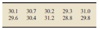
Construct a stem-and-leaf diagram for these data with
- a. one line per stem.
- b. two lines per stem.
- c. Which stem-and-leaf diagram do you find more useful? Why?
Expert Solution & Answer
Want to see the full answer?
Check out a sample textbook solution
Students have asked these similar questions
a small pond contains eight catfish and six bluegill. If seven fish are caught at random, what is the probability that exactly five catfish have been caught?
23 The line graph in the following figure shows
Revenue ($ millions)
one company's revenues over time. Explain
why this graph is misleading and what you
can do to fix the problem.
700
60-
50-
40
30
Line Graph of Revenue
20-
101
1950
1970
1975 1980 1985
Year
1990
2000
d of the
20
respectively.
Interpret the shape, center and spread of the
following box plot.
14
13
12
11
10
6
T
89
7
9
5.
治
Chapter 2 Solutions
Introductory Statistics (10th Edition)
Ch. 2.1 - Give an example, other than those presented in...Ch. 2.1 - Explain the meaning of a. qualitative variable. b....Ch. 2.1 - Explain the meaning of a. qualitative data. b....Ch. 2.1 - Provide a reason why the classification of data is...Ch. 2.1 - Of the variables you have studied so far, which...Ch. 2.1 - For each part of Exercises 2.62.11, classify the...Ch. 2.1 - Earthquakes. The U.S. Geological Survey monitors...Ch. 2.1 - Top 10 IPOs. An online article from the Washington...Ch. 2.1 - Earnings from the Crypt. On the Celebrity NetWorth...Ch. 2.1 - World University Rankings. The Times Higher...
Ch. 2.1 - Recording Industry Statistics. The Recording...Ch. 2.1 - RBI Kings. As reported on MLB.com, the five...Ch. 2.1 - Top Broadcast Shows. As reported in Primetime...Ch. 2.1 - The Fulbright Program. The U.S. governments...Ch. 2.1 - Top 10 Green Cars. The following table presents...Ch. 2.1 - Ordinal Data. Another important type of data is...Ch. 2.2 - What is a frequency distribution of qualitative...Ch. 2.2 - Explain the difference between a. frequency and...Ch. 2.2 - Answer true or false to each of the statements in...Ch. 2.2 - In Exercises 2.202.25, we have presented some...Ch. 2.2 - Prob. 21ECh. 2.2 - In Exercises 2.202.25, we have presented some...Ch. 2.2 - Prob. 23ECh. 2.2 - In Exercises 2.202.25, we have presented some...Ch. 2.2 - In Exercises 2.202.25, we have presented some...Ch. 2.2 - For each data set in Exercises 2.262.31, a....Ch. 2.2 - For each data set in Exercises 2.262.31, a....Ch. 2.2 - For each data set in Exercises 2.262.31, a....Ch. 2.2 - For each data set in Exercises 2.262.31, a....Ch. 2.2 - For each data set in Exercises 2.262.31, a....Ch. 2.2 - For each data set in Exercises 2.262.31, a....Ch. 2.2 - In each of Exercises 2.322.37, we have presented a...Ch. 2.2 - In each of Exercises 2.322.37, we have presented a...Ch. 2.2 - In each of Exercises 2.322.37, we have presented a...Ch. 2.2 - In each of Exercises 2.322.37, we have presented a...Ch. 2.2 - In each of Exercises 2.322.37, we have presented a...Ch. 2.2 - Prob. 37ECh. 2.2 - Health Status. The National Center for Health...Ch. 2.2 - In Exercises 2.392.41, use the technology of your...Ch. 2.2 - Prob. 40ECh. 2.2 - In Exercises 2.392.41, use the technology of your...Ch. 2.3 - Identify an important reason for grouping data.Ch. 2.3 - Do the concepts of class limits, marks, cutpoints,...Ch. 2.3 - State three of the most important guidelines in...Ch. 2.3 - With regard to grouping quantitative data into...Ch. 2.3 - For quantitative data, we examined three types of...Ch. 2.3 - We used slightly different methods for determining...Ch. 2.3 - Explain the difference between a frequency...Ch. 2.3 - Explain the advantages and disadvantages of...Ch. 2.3 - For data that are grouped in classes based on more...Ch. 2.3 - Discuss the relative advantages and disadvantages...Ch. 2.3 - Suppose that you have a data set that contains a...Ch. 2.3 - Suppose that you have constructed a stem-and-leaf...Ch. 2.3 - In each of Exercises 2.542.59, we have presented a...Ch. 2.3 - In each of Exercises 2.542.59, we have presented a...Ch. 2.3 - In each of Exercises 2.542.59, we have presented a...Ch. 2.3 - In each of Exercises 2.542.59, we have presented a...Ch. 2.3 - Prob. 58ECh. 2.3 - In each of Exercises 2.542.59, we have presented a...Ch. 2.3 - Prob. 60ECh. 2.3 - Prob. 61ECh. 2.3 - In Exercises 2.602.71, we have presented some...Ch. 2.3 - In Exercises 2.602.71, we have presented some...Ch. 2.3 - In Exercises 2.602.71, we have presented some...Ch. 2.3 - In Exercises 2.602.71, we have presented some...Ch. 2.3 - Prob. 66ECh. 2.3 - In Exercises 2.602.71, we have presented some...Ch. 2.3 - In Exercises 2.602.71, we have presented some...Ch. 2.3 - Prob. 69ECh. 2.3 - In Exercises 2.602.71, we have presented some...Ch. 2.3 - In Exercises 2.602.71, we have presented some...Ch. 2.3 - Prob. 72ECh. 2.3 - In each of Exercises 2.722.75, construct a dotplot...Ch. 2.3 - Prob. 74ECh. 2.3 - In each of Exercises 2.722.75, construct a dotplot...Ch. 2.3 - In each of Exercises 2.762.79, construct a...Ch. 2.3 - Prob. 77ECh. 2.3 - In each of Exercises 2.762.79, construct a...Ch. 2.3 - Prob. 79ECh. 2.3 - Prob. 80ECh. 2.3 - For each data set in Exercises 2.802.91, use the...Ch. 2.3 - For each data set in Exercises 2.802.91, use the...Ch. 2.3 - For each data set in Exercises 2.802.91, use the...Ch. 2.3 - For each data set in Exercises 2.802.91, use the...Ch. 2.3 - For each data set in Exercises 2.802.91, use the...Ch. 2.3 - For each data set in Exercises 2.802.91, use the...Ch. 2.3 - Prob. 87ECh. 2.3 - Prob. 88ECh. 2.3 - Prob. 89ECh. 2.3 - Prob. 90ECh. 2.3 - Prob. 91ECh. 2.3 - Prob. 92ECh. 2.3 - Age of Passenger Cars. According to R. L. Polk ...Ch. 2.3 - Stressed-Out Bus Drivers. Frustrated passengers,...Ch. 2.3 - Acute Postoperative Days. Several neurosurgeons...Ch. 2.3 - MMs. In the article Sweetening StatisticsWhat MMs...Ch. 2.3 - Women in the Workforce. In an issue of Science...Ch. 2.3 - Process Capability. R. Morris and E. Watson...Ch. 2.3 - University Patents. The number of patents a...Ch. 2.3 - Prob. 100ECh. 2.3 - Prob. 101ECh. 2.3 - Adjusted Gross Incomes. The Internal Revenue...Ch. 2.3 - Cholesterol Levels. According to the National...Ch. 2.3 - Hospital Beds. The number of hospital beds...Ch. 2.3 - Parkinsons Disease. Parkinsons disease affects...Ch. 2.3 - The Great White Shark. In an article titled Great...Ch. 2.3 - The Beatles. In the article, Length of The Beatles...Ch. 2.3 - High School Completion. As reported by the U.S....Ch. 2.3 - Prob. 109ECh. 2.3 - Body Temperature. A study by researchers at the...Ch. 2.3 - Exam Scores. The exam scores for the students in...Ch. 2.3 - Prob. 112ECh. 2.3 - Prob. 113ECh. 2.3 - Age and Gender. The following bivariate data on...Ch. 2.3 - Prob. 115ECh. 2.3 - Clocking the Cheetah. Construct a...Ch. 2.3 - Prob. 117ECh. 2.3 - Residential Energy Consumption. Refer to the...Ch. 2.3 - Prob. 119ECh. 2.3 - Cardiovascular Hospitalizations. The Florida State...Ch. 2.3 - Prob. 121ECh. 2.4 - In each of Exercises 2.1222.127, explain the...Ch. 2.4 - In each of Exercises 2.1222.127, explain the...Ch. 2.4 - In each of Exercises 2.1222.127, explain the...Ch. 2.4 - Prob. 125ECh. 2.4 - Prob. 126ECh. 2.4 - Prob. 127ECh. 2.4 - Prob. 128ECh. 2.4 - Suppose that a variable of a population has a...Ch. 2.4 - Prob. 130ECh. 2.4 - Identify and sketch three distribution shapes that...Ch. 2.4 - Prob. 132ECh. 2.4 - In each of Exercises 2.1322.139, we have drawn a...Ch. 2.4 - In each of Exercises 2.1322.139, we have drawn a...Ch. 2.4 - In each of Exercises 2.1322.139, we have drawn a...Ch. 2.4 - In each of Exercises 2.1322.139, we have drawn a...Ch. 2.4 - In each of Exercises 2.1322.139, we have drawn a...Ch. 2.4 - In each of Exercises 2.1322.139, we have drawn a...Ch. 2.4 - Prob. 139ECh. 2.4 - In each of Exercises 2.1402.149, we have provided...Ch. 2.4 - In each of Exercises 2.1402.149, we have provided...Ch. 2.4 - Prob. 142ECh. 2.4 - In each of Exercises 2.1402.149, we have provided...Ch. 2.4 - In each of Exercises 2.1402.149, we have provided...Ch. 2.4 - In each of Exercises 2.1402.149, we have provided...Ch. 2.4 - In each of Exercises 2.1402.149, we have provided...Ch. 2.4 - Prob. 147ECh. 2.4 - Prob. 148ECh. 2.4 - Prob. 149ECh. 2.4 - Old Faithful. Old Faithful is a geyser in...Ch. 2.4 - SnowGoose Nests. In the article Trophic...Ch. 2.4 - Prob. 152ECh. 2.4 - In each of Exercises 2.1522.157, a. use the...Ch. 2.4 - In each of Exercises 2.1522.157, a. use the...Ch. 2.4 - Prob. 155ECh. 2.4 - In each of Exercises 2.1522.157, a. use the...Ch. 2.4 - In each of Exercises 2.1522.157, a. use the...Ch. 2.4 - Standard Normal Distribution. One of the most...Ch. 2.5 - Give one reason why constructing and reading...Ch. 2.5 - Prob. 163ECh. 2.5 - Reading Skills. Each year the director of the...Ch. 2.5 - Americas Melting Pot. The U.S. Census Bureau...Ch. 2.5 - Prob. 167ECh. 2.5 - Drunk-Driving Fatalities. Drunk-driving fatalities...Ch. 2.5 - Prob. 169ECh. 2.5 - Prob. 170ECh. 2.5 - Prob. 171ECh. 2 - This problem is about variables. a. What is a...Ch. 2 - This problem is about data. a. What are data? b....Ch. 2 - For a qualitative data set, what is a a. frequency...Ch. 2 - What is the relationship between a frequency or...Ch. 2 - Identify two main types of graphical displays that...Ch. 2 - In a bar chart, unlike in a histogram, the bars do...Ch. 2 - Some users of statistics prefer pie charts to bar...Ch. 2 - When is the use of single-value grouping...Ch. 2 - A quantitative data set has been grouped by using...Ch. 2 - A quantitative data set has been grouped by using...Ch. 2 - A quantitative data set has been grouped by using...Ch. 2 - A quantitative data set has been grouped by using...Ch. 2 - Explain the relative positioning of the bars in a...Ch. 2 - Sketch the curve corresponding to each of the...Ch. 2 - Draw a smooth curve that represents a symmetric...Ch. 2 - Prob. 16RPCh. 2 - Largest Hydroelectric Plants. According to...Ch. 2 - DVD Players. Refer to Example 2.16 on page 60. a....Ch. 2 - Inauguration Ages. From the Information Please...Ch. 2 - Inauguration Ages. Refer to Problem 19. Construct...Ch. 2 - Prob. 21RPCh. 2 - Prob. 22RPCh. 2 - Busy Bank Tellers. The Prescott National Bank has...Ch. 2 - On-Time Arrivals. The Air Travel Consumer Report...Ch. 2 - Old Ballplayers. From the ESPN Web site, we...Ch. 2 - Prob. 26RPCh. 2 - U.S. Divisions. The U.S. Census Bureau divides the...Ch. 2 - Prob. 28RPCh. 2 - Prob. 29RPCh. 2 - Hair and Eye Color. In the article Graphical...Ch. 2 - Prob. 31RPCh. 2 - In Problems 3133, a. identify the population and...Ch. 2 - In Problems 3133, a. identify the population and...Ch. 2 - UWEC UNDERGRADUATES Recall from Chapter 1 (see...Ch. 2 - Recall that, each year, Forbes magazine publishes...
Knowledge Booster


Learn more about
Need a deep-dive on the concept behind this application? Look no further. Learn more about this topic, statistics and related others by exploring similar questions and additional content below.Similar questions
- F Make a box plot from the five-number summary: 100, 105, 120, 135, 140. harrow_forward14 Is the standard deviation affected by skewed data? If so, how? foldarrow_forwardFrequency 15 Suppose that your friend believes his gambling partner plays with a loaded die (not fair). He shows you a graph of the outcomes of the games played with this die (see the following figure). Based on this graph, do you agree with this person? Why or why not? 65 Single Die Outcomes: Graph 1 60 55 50 45 40 1 2 3 4 Outcome 55 6arrow_forward
- lie y H 16 The first month's telephone bills for new customers of a certain phone company are shown in the following figure. The histogram showing the bills is misleading, however. Explain why, and suggest a solution. Frequency 140 120 100 80 60 40 20 0 0 20 40 60 80 Telephone Bill ($) 100 120arrow_forward25 ptical rule applies because t Does the empirical rule apply to the data set shown in the following figure? Explain. 2 6 5 Frequency 3 сл 2 1 0 2 4 6 8 00arrow_forward24 Line graphs typically connect the dots that represent the data values over time. If the time increments between the dots are large, explain why the line graph can be somewhat misleading.arrow_forward
- 17 Make a box plot from the five-number summary: 3, 4, 7, 16, 17. 992) waarrow_forward12 10 - 8 6 4 29 0 Interpret the shape, center and spread of the following box plot. brill smo slob.nl bagharrow_forwardSuppose that a driver's test has a mean score of 7 (out of 10 points) and standard deviation 0.5. a. Explain why you can reasonably assume that the data set of the test scores is mound-shaped. b. For the drivers taking this particular test, where should 68 percent of them score? c. Where should 95 percent of them score? d. Where should 99.7 percent of them score? Sarrow_forward
- 13 Can the mean of a data set be higher than most of the values in the set? If so, how? Can the median of a set be higher than most of the values? If so, how? srit to estaarrow_forwardA random variable X takes values 0 and 1 with probabilities q and p, respectively, with q+p=1. find the moment generating function of X and show that all the moments about the origin equal p. (Note- Please include as much detailed solution/steps in the solution to understand, Thank you!)arrow_forward1 (Expected Shortfall) Suppose the price of an asset Pt follows a normal random walk, i.e., Pt = Po+r₁ + ... + rt with r₁, r2,... being IID N(μ, o²). Po+r1+. ⚫ Suppose the VaR of rt is VaRq(rt) at level q, find the VaR of the price in T days, i.e., VaRq(Pt – Pt–T). - • If ESq(rt) = A, find ES₁(Pt – Pt–T).arrow_forward
arrow_back_ios
SEE MORE QUESTIONS
arrow_forward_ios
Recommended textbooks for you
 Glencoe Algebra 1, Student Edition, 9780079039897...AlgebraISBN:9780079039897Author:CarterPublisher:McGraw Hill
 Functions and Change: A Modeling Approach to Coll...AlgebraISBN:9781337111348Author:Bruce Crauder, Benny Evans, Alan NoellPublisher:Cengage Learning
 Big Ideas Math A Bridge To Success Algebra 1: Stu...AlgebraISBN:9781680331141Author:HOUGHTON MIFFLIN HARCOURTPublisher:Houghton Mifflin Harcourt
Glencoe Algebra 1, Student Edition, 9780079039897...
Algebra
ISBN:9780079039897
Author:Carter
Publisher:McGraw Hill
Functions and Change: A Modeling Approach to Coll...
Algebra
ISBN:9781337111348
Author:Bruce Crauder, Benny Evans, Alan Noell
Publisher:Cengage Learning
Big Ideas Math A Bridge To Success Algebra 1: Stu...
Algebra
ISBN:9781680331141
Author:HOUGHTON MIFFLIN HARCOURT
Publisher:Houghton Mifflin Harcourt
F- Test or F- statistic (F- Test of Equality of Variance); Author: Prof. Arvind Kumar Sing;https://www.youtube.com/watch?v=PdUt7InTyc8;License: Standard Youtube License
Statistics 101: F-ratio Test for Two Equal Variances; Author: Brandon Foltz;https://www.youtube.com/watch?v=UWQO4gX7-lE;License: Standard YouTube License, CC-BY
Hypothesis Testing and Confidence Intervals (FRM Part 1 – Book 2 – Chapter 5); Author: Analystprep;https://www.youtube.com/watch?v=vth3yZIUlGQ;License: Standard YouTube License, CC-BY
Understanding the Levene's Test for Equality of Variances in SPSS; Author: Dr. Todd Grande;https://www.youtube.com/watch?v=udJr8V2P8Xo;License: Standard Youtube License