
Modern Business Statistics with Microsoft Office Excel (with XLSTAT Education Edition Printed Access Card)
6th Edition
ISBN: 9780357228708
Author: David R. Anderson; Dennis J. Sweeney; Thomas A. Williams
Publisher: Cengage Learning US
expand_more
expand_more
format_list_bulleted
Concept explainers
Videos
Textbook Question
Chapter 2.3, Problem 32E
Household Income Levels. The following crosstabulation shows the number of households (1000s) in each of the four regions of the United States and the number of households at each income level (U.S. Census Bureau website, https://www.census.gov/data/tables/time-series/demo/income-poverty/cps-hinc.html).
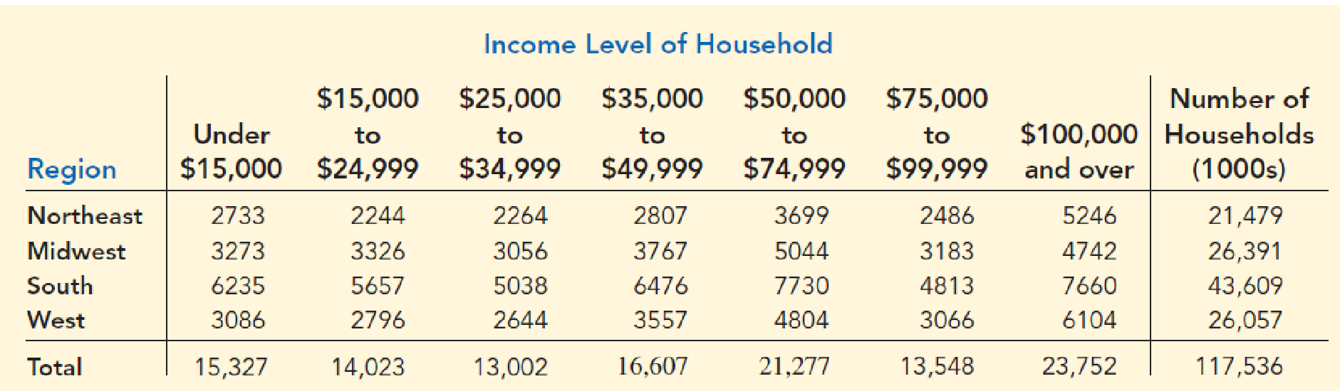
- a. Compute the row percentages and identify the percent frequency distributions of income for households in each region.
- b. What percentage of households in the West region have an income level of $50,000 or more? What percentage of households in the South region have an income level of $50,000 or more?
- c. Construct percent frequency histograms for each region of households. Do any relationships between regions and income level appear to be evident in your findings?
- d. Compute the column percentages. What information do the column percentages provide?
- e. What percent of households with a household income of $100,000 and over are from the South region? What percentage of households from the South region have a household income of $100,000 and over? Why are these two percentages different?
Expert Solution & Answer
Want to see the full answer?
Check out a sample textbook solution
Students have asked these similar questions
Install RStudio: Begin by installing RStudio on your computer. If you haven't done so, please refer to the official RStudio website for download and installation instructions.
Watch the Tutorial Video: Watch the provided video tutorial that explains how to run RStudio. Pay close attention to the steps for opening and managing data files. https://www.youtube.com/watch?v=RhJp6vSZ7z0
Open RStudio: Once RStudio is installed, open the application.
Load the Dataset: In RStudio, open a data file named "mtcars". To do this, type the command mtcars in the script editor and run the command.
Attach the Data: Next, attach the dataset using the command attach(mtcars).
Examine the Variables: Carefully review and note the names of all variables in the dataset. Examples of these variables include:
Mileage (mpg)
Number of Cylinders (cyl)
Displacement (disp)
Horsepower (hp)
Research: Google to understand these variables.
Statistical Analysis: Select mpg variable, and perform the following…
A marketing professor has surveyed the students at her university to better understand attitudes towards PPT usage for higher education. To be able to make inferences to the entire student body, the sample drawn needs to represent the university’s student population on all key characteristics. The table below shows the five key student demographic variables. The professor found the breakdown of the overall student body in the university’s fact book posted online.
A non-parametric chi-square test was used to test the sample demographics against the population percentages shown in the table above. Review the output for the five chi-square tests on the following pages and answer the five questions:
Based on the chi-square test, which sample variables adequately represent the university’s student population and which ones do not? Support your answer by providing the p-value of the chi-square test and explaining what it means.
Using the results from Question 1, make recommendation for…
Chapter 2 Solutions
Modern Business Statistics with Microsoft Office Excel (with XLSTAT Education Edition Printed Access Card)
Ch. 2.1 - Methods
1. The response to a question has three...Ch. 2.1 - 2. A partial relative frequency distribution is...Ch. 2.1 - A questionnaire provides 58 Yes, 42 No, and 20...Ch. 2.1 -
For the 2010–2011 viewing season, the top five...Ch. 2.1 -
In alphabetical order, the six most common last...Ch. 2.1 - Top Rated Television Show Networks. Nielsen Media...Ch. 2.1 - Airline Customer Satisfaction Survey. Many...Ch. 2.1 - Prob. 8ECh. 2.1 - Prob. 9ECh. 2.1 -
VirtualTourist provides ratings for hotels...
Ch. 2.2 - 11. Consider the following data.
Develop a...Ch. 2.2 - 12. Consider the following frequency...Ch. 2.2 - Construct a histogram for the data in exercise...Ch. 2.2 - Prob. 14ECh. 2.2 - Construct a stem-and-leaf display for the...Ch. 2.2 - Construct a stem-and-leaf display for the...Ch. 2.2 - Applications
17. A doctor’s office staff studied...Ch. 2.2 - NBA Total Player Ratings. CBSSports.com developed...Ch. 2.2 - Prob. 19ECh. 2.2 - CEO Time in Meetings. The London School of...Ch. 2.2 - Quantcast.com provides the number of people from...Ch. 2.2 - Top U.S. Franchises. Entrepreneur magazine ranks...Ch. 2.2 - Prob. 24ECh. 2.2 - Best Paying College Degrees. Each year America.EDU...Ch. 2.2 - Prob. 26ECh. 2.3 - The following data are for 30 observations...Ch. 2.3 - The following observations are for two...Ch. 2.3 - Daytona 500 Automobile Makes Average Speeds. The...Ch. 2.3 - Daytona 500 Average Speeds of Winners. The...Ch. 2.3 - 31. Recently, management at Oak Tree Golf Course...Ch. 2.3 - Household Income Levels. The following...Ch. 2.3 - 33. Each year Forbes ranks the world’s most...Ch. 2.3 - Prob. 34ECh. 2.3 -
The U.S. Department of Energy's Fuel Economy...Ch. 2.4 - The following 20 observations are for two...Ch. 2.4 - Prob. 37ECh. 2.4 - The following crosstabulation summarizes the data...Ch. 2.4 - Driving Speed and Fuel Efficiency. A study on...Ch. 2.4 - The DATAfile Snow contains average annual snowfall...Ch. 2.4 - Hypertension and Heart Disease. People often wait...Ch. 2.4 -
Smartphones are mobile phones with Internet,...Ch. 2.4 - Store Managers Time Study. The Northwest regional...Ch. 2 - SAT Scores. The SAT is a standardized test used by...Ch. 2 - Median Household Incomes. The file MedianHousehold...Ch. 2 - State Populations. Data showing the population by...Ch. 2 - Startup Company Funds. According to the Wall...Ch. 2 - Complaints Reported to BBB. Consumer complaints...Ch. 2 - Stock Price Volatility. The term “beta” refers to...Ch. 2 - Education Level and Household Income. The U.S....Ch. 2 - Prob. 51SECh. 2 - Best Places to Work. Fortune magazine publishes an...Ch. 2 - Prob. 53SECh. 2 - Prob. 54SECh. 2 - Prob. 55SECh. 2 - Prob. 56SECh. 2 -
Google has changed its strategy with regard to...Ch. 2 -
A zoo has categorized its visitors into three...Ch. 2 - Pelican Stores, a division of National Clothing,...Ch. 2 -
Motion Picture Industry
The motion picture...Ch. 2 - Cincinnati, Ohio, also known as the Queen City,...Ch. 2 - Jon Weideman, first shift foreman for Cut-Rate...
Knowledge Booster


Learn more about
Need a deep-dive on the concept behind this application? Look no further. Learn more about this topic, statistics and related others by exploring similar questions and additional content below.Similar questions
- A retail chain is interested in determining whether a digital video point-of-purchase (POP) display would stimulate higher sales for a brand advertised compared to the standard cardboard point-of-purchase display. To test this, a one-shot static group design experiment was conducted over a four-week period in 100 different stores. Fifty stores were randomly assigned to the control treatment (standard display) and the other 50 stores were randomly assigned to the experimental treatment (digital display). Compare the sales of the control group (standard POP) to the experimental group (digital POP). What were the average sales for the standard POP display (control group)? What were the sales for the digital display (experimental group)? What is the (mean) difference in sales between the experimental group and control group? List the null hypothesis being tested. Do you reject or retain the null hypothesis based on the results of the independent t-test? Was the difference between the…arrow_forwardWhat were the average sales for the four weeks prior to the experiment? What were the sales during the four weeks when the stores used the digital display? What is the mean difference in sales between the experimental and regular POP time periods? State the null hypothesis being tested by the paired sample t-test. Do you reject or retain the null hypothesis? At a 95% significance level, was the difference significant? Explain why or why not using the results from the paired sample t-test. Should the manager of the retail chain install new digital displays in each store? Justify your answer.arrow_forwardA retail chain is interested in determining whether a digital video point-of-purchase (POP) display would stimulate higher sales for a brand advertised compared to the standard cardboard point-of-purchase display. To test this, a one-shot static group design experiment was conducted over a four-week period in 100 different stores. Fifty stores were randomly assigned to the control treatment (standard display) and the other 50 stores were randomly assigned to the experimental treatment (digital display). Compare the sales of the control group (standard POP) to the experimental group (digital POP). What were the average sales for the standard POP display (control group)? What were the sales for the digital display (experimental group)? What is the (mean) difference in sales between the experimental group and control group? List the null hypothesis being tested. Do you reject or retain the null hypothesis based on the results of the independent t-test? Was the difference between the…arrow_forward
- Question 4 An article in Quality Progress (May 2011, pp. 42-48) describes the use of factorial experiments to improve a silver powder production process. This product is used in conductive pastes to manufacture a wide variety of products ranging from silicon wafers to elastic membrane switches. Powder density (g/cm²) and surface area (cm/g) are the two critical characteristics of this product. The experiments involved three factors: reaction temperature, ammonium percentage, stirring rate. Each of these factors had two levels, and the design was replicated twice. The design is shown in Table 3. A222222222222233 Stir Rate (RPM) Ammonium (%) Table 3: Silver Powder Experiment from Exercise 13.23 Temperature (°C) Density Surface Area 100 8 14.68 0.40 100 8 15.18 0.43 30 100 8 15.12 0.42 30 100 17.48 0.41 150 7.54 0.69 150 8 6.66 0.67 30 150 8 12.46 0.52 30 150 8 12.62 0.36 100 40 10.95 0.58 100 40 17.68 0.43 30 100 40 12.65 0.57 30 100 40 15.96 0.54 150 40 8.03 0.68 150 40 8.84 0.75 30 150…arrow_forward- + ++ Table 2: Crack Experiment for Exercise 2 A B C D Treatment Combination (1) Replicate I II 7.037 6.376 14.707 15.219 |++++ 1 བྱ॰༤༠སྦྱོ སྦྱོཋཏྟཱུ a b ab 11.635 12.089 17.273 17.815 с ас 10.403 10.151 4.368 4.098 bc abc 9.360 9.253 13.440 12.923 d 8.561 8.951 ad 16.867 17.052 bd 13.876 13.658 abd 19.824 19.639 cd 11.846 12.337 acd 6.125 5.904 bcd 11.190 10.935 abcd 15.653 15.053 Question 3 Continuation of Exercise 2. One of the variables in the experiment described in Exercise 2, heat treatment method (C), is a categorical variable. Assume that the remaining factors are continuous. (a) Write two regression models for predicting crack length, one for each level of the heat treatment method variable. What differences, if any, do you notice in these two equations? (b) Generate appropriate response surface contour plots for the two regression models in part (a). (c) What set of conditions would you recommend for the factors A, B, and D if you use heat treatment method C = +? (d) Repeat…arrow_forwardQuestion 2 A nickel-titanium alloy is used to make components for jet turbine aircraft engines. Cracking is a potentially serious problem in the final part because it can lead to nonrecoverable failure. A test is run at the parts producer to determine the effect of four factors on cracks. The four factors are: pouring temperature (A), titanium content (B), heat treatment method (C), amount of grain refiner used (D). Two replicates of a 24 design are run, and the length of crack (in mm x10-2) induced in a sample coupon subjected to a standard test is measured. The data are shown in Table 2. 1 (a) Estimate the factor effects. Which factor effects appear to be large? (b) Conduct an analysis of variance. Do any of the factors affect cracking? Use a = 0.05. (c) Write down a regression model that can be used to predict crack length as a function of the significant main effects and interactions you have identified in part (b). (d) Analyze the residuals from this experiment. (e) Is there an…arrow_forward
- A 24-1 design has been used to investigate the effect of four factors on the resistivity of a silicon wafer. The data from this experiment are shown in Table 4. Table 4: Resistivity Experiment for Exercise 5 Run A B с D Resistivity 1 23 2 3 4 5 6 7 8 9 10 11 12 I+I+I+I+Oooo 0 0 ||++TI++o000 33.2 4.6 31.2 9.6 40.6 162.4 39.4 158.6 63.4 62.6 58.7 0 0 60.9 3 (a) Estimate the factor effects. Plot the effect estimates on a normal probability scale. (b) Identify a tentative model for this process. Fit the model and test for curvature. (c) Plot the residuals from the model in part (b) versus the predicted resistivity. Is there any indication on this plot of model inadequacy? (d) Construct a normal probability plot of the residuals. Is there any reason to doubt the validity of the normality assumption?arrow_forwardStem1: 1,4 Stem 2: 2,4,8 Stem3: 2,4 Stem4: 0,1,6,8 Stem5: 0,1,2,3,9 Stem 6: 2,2 What’s the Min,Q1, Med,Q3,Max?arrow_forwardAre the t-statistics here greater than 1.96? What do you conclude? colgPA= 1.39+0.412 hsGPA (.33) (0.094) Find the P valuearrow_forward
- A poll before the elections showed that in a given sample 79% of people vote for candidate C. How many people should be interviewed so that the pollsters can be 99% sure that from 75% to 83% of the population will vote for candidate C? Round your answer to the whole number.arrow_forwardSuppose a random sample of 459 married couples found that 307 had two or more personality preferences in common. In another random sample of 471 married couples, it was found that only 31 had no preferences in common. Let p1 be the population proportion of all married couples who have two or more personality preferences in common. Let p2 be the population proportion of all married couples who have no personality preferences in common. Find a95% confidence interval for . Round your answer to three decimal places.arrow_forwardA history teacher interviewed a random sample of 80 students about their preferences in learning activities outside of school and whether they are considering watching a historical movie at the cinema. 69 answered that they would like to go to the cinema. Let p represent the proportion of students who want to watch a historical movie. Determine the maximal margin of error. Use α = 0.05. Round your answer to three decimal places. arrow_forward
arrow_back_ios
SEE MORE QUESTIONS
arrow_forward_ios
Recommended textbooks for you
 Glencoe Algebra 1, Student Edition, 9780079039897...AlgebraISBN:9780079039897Author:CarterPublisher:McGraw Hill
 Holt Mcdougal Larson Pre-algebra: Student Edition...AlgebraISBN:9780547587776Author:HOLT MCDOUGALPublisher:HOLT MCDOUGAL
 Big Ideas Math A Bridge To Success Algebra 1: Stu...AlgebraISBN:9781680331141Author:HOUGHTON MIFFLIN HARCOURTPublisher:Houghton Mifflin Harcourt
Glencoe Algebra 1, Student Edition, 9780079039897...
Algebra
ISBN:9780079039897
Author:Carter
Publisher:McGraw Hill
Holt Mcdougal Larson Pre-algebra: Student Edition...
Algebra
ISBN:9780547587776
Author:HOLT MCDOUGAL
Publisher:HOLT MCDOUGAL
Big Ideas Math A Bridge To Success Algebra 1: Stu...
Algebra
ISBN:9781680331141
Author:HOUGHTON MIFFLIN HARCOURT
Publisher:Houghton Mifflin Harcourt
The Shape of Data: Distributions: Crash Course Statistics #7; Author: CrashCourse;https://www.youtube.com/watch?v=bPFNxD3Yg6U;License: Standard YouTube License, CC-BY
Shape, Center, and Spread - Module 20.2 (Part 1); Author: Mrmathblog;https://www.youtube.com/watch?v=COaid7O_Gag;License: Standard YouTube License, CC-BY
Shape, Center and Spread; Author: Emily Murdock;https://www.youtube.com/watch?v=_YyW0DSCzpM;License: Standard Youtube License