
Essentials of Statistics, Loose-Leaf Edition PLUS MyLab Statistics with Pearson eText -- Access Card Package (6th Edition)
6th Edition
ISBN: 9780135245729
Author: Mario F. Triola
Publisher: PEARSON
expand_more
expand_more
format_list_bulleted
Videos
Textbook Question
Chapter 2.3, Problem 10BSC
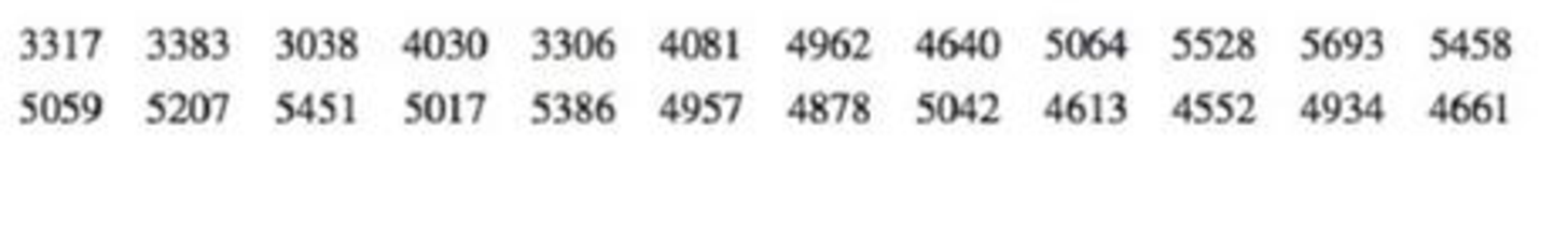
Time-Series Graphs. In Exercises 9 and 10, construct the time-series graph.
10. Home Runs Listed below are the numbers of home runs in Major League Baseball for each year beginning with 1990 (listed in order by row). Is there a trend?
Expert Solution & Answer
Want to see the full answer?
Check out a sample textbook solution
Students have asked these similar questions
A retail chain is interested in determining whether a digital video point-of-purchase (POP) display would stimulate higher sales for a brand advertised compared to the standard cardboard point-of-purchase display. To test this, a one-shot static group design experiment was conducted over a four-week period in 100 different stores. Fifty stores were randomly assigned to the control treatment (standard display) and the other 50 stores were randomly assigned to the experimental treatment (digital display). Compare the sales of the control group (standard POP) to the experimental group (digital POP).
What were the average sales for the standard POP display (control group)?
What were the sales for the digital display (experimental group)?
What is the (mean) difference in sales between the experimental group and control group?
List the null hypothesis being tested.
Do you reject or retain the null hypothesis based on the results of the independent t-test?
Was the difference between the…
What were the average sales for the four weeks prior to the experiment?
What were the sales during the four weeks when the stores used the digital display?
What is the mean difference in sales between the experimental and regular POP time periods?
State the null hypothesis being tested by the paired sample t-test.
Do you reject or retain the null hypothesis?
At a 95% significance level, was the difference significant? Explain why or why not using the results from the paired sample t-test.
Should the manager of the retail chain install new digital displays in each store? Justify your answer.
A retail chain is interested in determining whether a digital video point-of-purchase (POP) display would stimulate higher sales for a brand advertised compared to the standard cardboard point-of-purchase display. To test this, a one-shot static group design experiment was conducted over a four-week period in 100 different stores. Fifty stores were randomly assigned to the control treatment (standard display) and the other 50 stores were randomly assigned to the experimental treatment (digital display). Compare the sales of the control group (standard POP) to the experimental group (digital POP).
What were the average sales for the standard POP display (control group)?
What were the sales for the digital display (experimental group)?
What is the (mean) difference in sales between the experimental group and control group?
List the null hypothesis being tested.
Do you reject or retain the null hypothesis based on the results of the independent t-test?
Was the difference between the…
Chapter 2 Solutions
Essentials of Statistics, Loose-Leaf Edition PLUS MyLab Statistics with Pearson eText -- Access Card Package (6th Edition)
Ch. 2.1 - McDonalds Dinner Service Times Refer 10 the...Ch. 2.1 - McDonalds Dinner Service Times Refer to the...Ch. 2.1 - Relative Frequency Distribution Use percentages to...Ch. 2.1 - Whats Wrong? Heights of adult males are known to...Ch. 2.1 - In Exercise 58, identify the class width, class...Ch. 2.1 - In Exercises 58, identify the class width, class...Ch. 2.1 - In Exercises 58, identify the class width, class...Ch. 2.1 - In Exercises 58, identify the class width, class...Ch. 2.1 - Normal Distributions. In Exercises 9 and 10, using...Ch. 2.1 - Normal Distributions. In Exercises 9 and 10, using...
Ch. 2.1 - Constructing Frequency Distributions. In Exercises...Ch. 2.1 - Constructing Frequency Distributions. In Exercises...Ch. 2.1 - Constructing Frequency Distributions. In Exercises...Ch. 2.1 - Burger King Dinner Service Times Refer to Data Set...Ch. 2.1 - Wendys Lunch Service Times Refer to Data Set 25...Ch. 2.1 - Wendys Dinner Service Times Refer to Data Set 25...Ch. 2.1 - Analysis of Last Digits Heights of statistics...Ch. 2.1 - Analysis of Last Digits Weights of respondents...Ch. 2.1 - Oscar Winners Construct one table (similar to...Ch. 2.1 - Blood Platelet Counts Construct one table (similar...Ch. 2.1 - Cumulative Frequency Distributions. In Exercises...Ch. 2.1 - Cumulative Frequency Distributions. In Exercises...Ch. 2.1 - Categorical Data. In Exercises 23 and 24, use the...Ch. 2.1 - Categorical Data. In Exercises 23 and 24, use the...Ch. 2.2 - Heights Heights of adult males are normally...Ch. 2.2 - More Heights The population of heights of adult...Ch. 2.2 - Blood Platelet Counts Listed below are blood...Ch. 2.2 - Blood Platelet Counts If we collect a sample of...Ch. 2.2 - Interpreting a Histogram. In Exercises 58, answer...Ch. 2.2 - Prob. 6BSCCh. 2.2 - Interpreting a Histogram. In Exercises 58, answer...Ch. 2.2 - Prob. 8BSCCh. 2.2 - Constructing Histograms. In Exercises 9-16,...Ch. 2.2 - Constructing Histograms. In Exercises 9-16,...Ch. 2.2 - Burger King Lunch Service Times Use the frequency...Ch. 2.2 - Burger King Dinner Service Times Use the frequency...Ch. 2.2 - Wendys Lunch Service Times Use the frequency...Ch. 2.2 - Wendys Dinner Service Times Use the frequency...Ch. 2.2 - Analysis of Last Digits Use the frequency...Ch. 2.2 - Analysis of Last Digits Use the frequency...Ch. 2.2 - Back-to-Back Relative Frequency Histograms When...Ch. 2.2 - Interpreting Normal Quantile Plots Which of the...Ch. 2.3 - Body Temperatures Listed below are body...Ch. 2.3 - Voluntary Response Data If we have a large...Ch. 2.3 - Ethics There are data showing that smoking is...Ch. 2.3 - CVDOT Section 2-1 introduced important...Ch. 2.3 - Dotplots. In Exercises 5 and 6, construct the...Ch. 2.3 - Diastolic Blood Pressure Listed below are...Ch. 2.3 - Stem plots. In Exercises 7 and 8, construct the...Ch. 2.3 - Stemplots. In Exercises 7 and 8, construct the...Ch. 2.3 - Time-Series Graphs. In Exercises 9 and 10,...Ch. 2.3 - Time-Series Graphs. In Exercises 9 and 10,...Ch. 2.3 - Pareto Charts. In Exercises 11 and 12 construct...Ch. 2.3 - Pareto Charts. In Exercises 11 and 12 construct...Ch. 2.3 - Pie Charts. In Exercises 13 and 14, construct the...Ch. 2.3 - Pie Charts. In Exercises 13 and 14, construct the...Ch. 2.3 - Frequency Polygon. In Exercises 15 and 16,...Ch. 2.3 - Frequency Polygon. In Exercises 15 and 16,...Ch. 2.3 - Self-Driving Vehicles In a survey of adults,...Ch. 2.3 - Deceptive Graphs. In Exercises 17-20, identify how...Ch. 2.3 - Deceptive Graphs. In Exercises 17-20, identify how...Ch. 2.3 - Deceptive Graphs. In Exercises 17-20, identify how...Ch. 2.3 - Expanded Stemplots A stemplot can be condensed by...Ch. 2.4 - Linear Correlation In this section we use r to...Ch. 2.4 - Causation A study has shown that there is a...Ch. 2.4 - Scanerplot What is a scatterplot and how does it...Ch. 2.4 - Estimating r For each of the following, estimate...Ch. 2.4 - Scatterplot. In Exercises 5-8, use the sample data...Ch. 2.4 - Scatterplot. In Exercises 5-8, use the sample data...Ch. 2.4 - Scatterplot. In Exercises 5-8, use the sample data...Ch. 2.4 - Scatterplot. In Exercises 5-8, use the sample data...Ch. 2.4 - Linear Correlation Coefficient In Exercises 9-12,...Ch. 2.4 - Linear Correlation Coefficient In Exercises 9-12,...Ch. 2.4 - Linear Correlation Coefficient In Exercises 9-12,...Ch. 2.4 - Using the data from Exercise 8 Heights of Fathers...Ch. 2.4 - Prob. 13BBCh. 2.4 - P-Values In Exercises 13-16, write a statement...Ch. 2.4 - P-Values In Exercises 13-16, write a statement...Ch. 2.4 - P-Values In Exercises 13-16, write a statement...Ch. 2 - Cookies Refer to the accompanying frequency...Ch. 2 - Cookies Using the same frequency distribution from...Ch. 2 - Cookies Using the same frequency distribution from...Ch. 2 - Cookies A stemplot of the same cookies summarized...Ch. 2 - Computers As a quality control manager at Texas...Ch. 2 - Distribution of Wealth In recent years, there has...Ch. 2 - Health Test In an investigation of a relationship...Ch. 2 - Lottery In Floridas Play 4 lottery game, four...Ch. 2 - Seatbelts The Beams Seatbelts company...Ch. 2 - Seatbelts A histogram is to be constructed from...Ch. 2 - Frequency Distribution of Body Temperatures...Ch. 2 - Histogram of Body Temperatures Construct the...Ch. 2 - Dotplot of Body Temperatures Construct a dotplot...Ch. 2 - Stemplot of Body Temperatures Construct a stemplot...Ch. 2 - Body Temperatures Listed below are the...Ch. 2 - Environment a. After collecting the average (mean)...Ch. 2 - Its Like Time Do This Exercise In a Marist survey...Ch. 2 - Whatever Use the same data from Exercise 7 to...Ch. 2 - In Exercises 1-6 refer to the data below, which...Ch. 2 - Frequency Distribution For the frequency...Ch. 2 - In Exercises 1-6, refer to the data below, which...Ch. 2 - In Exercises 1-6, refer to the data below, which...Ch. 2 - In Exercises 1-6, refer to the data below, which...Ch. 2 - Data Type a. The listed playing times are all...
Knowledge Booster


Learn more about
Need a deep-dive on the concept behind this application? Look no further. Learn more about this topic, statistics and related others by exploring similar questions and additional content below.Similar questions
- Question 4 An article in Quality Progress (May 2011, pp. 42-48) describes the use of factorial experiments to improve a silver powder production process. This product is used in conductive pastes to manufacture a wide variety of products ranging from silicon wafers to elastic membrane switches. Powder density (g/cm²) and surface area (cm/g) are the two critical characteristics of this product. The experiments involved three factors: reaction temperature, ammonium percentage, stirring rate. Each of these factors had two levels, and the design was replicated twice. The design is shown in Table 3. A222222222222233 Stir Rate (RPM) Ammonium (%) Table 3: Silver Powder Experiment from Exercise 13.23 Temperature (°C) Density Surface Area 100 8 14.68 0.40 100 8 15.18 0.43 30 100 8 15.12 0.42 30 100 17.48 0.41 150 7.54 0.69 150 8 6.66 0.67 30 150 8 12.46 0.52 30 150 8 12.62 0.36 100 40 10.95 0.58 100 40 17.68 0.43 30 100 40 12.65 0.57 30 100 40 15.96 0.54 150 40 8.03 0.68 150 40 8.84 0.75 30 150…arrow_forward- + ++ Table 2: Crack Experiment for Exercise 2 A B C D Treatment Combination (1) Replicate I II 7.037 6.376 14.707 15.219 |++++ 1 བྱ॰༤༠སྦྱོ སྦྱོཋཏྟཱུ a b ab 11.635 12.089 17.273 17.815 с ас 10.403 10.151 4.368 4.098 bc abc 9.360 9.253 13.440 12.923 d 8.561 8.951 ad 16.867 17.052 bd 13.876 13.658 abd 19.824 19.639 cd 11.846 12.337 acd 6.125 5.904 bcd 11.190 10.935 abcd 15.653 15.053 Question 3 Continuation of Exercise 2. One of the variables in the experiment described in Exercise 2, heat treatment method (C), is a categorical variable. Assume that the remaining factors are continuous. (a) Write two regression models for predicting crack length, one for each level of the heat treatment method variable. What differences, if any, do you notice in these two equations? (b) Generate appropriate response surface contour plots for the two regression models in part (a). (c) What set of conditions would you recommend for the factors A, B, and D if you use heat treatment method C = +? (d) Repeat…arrow_forwardQuestion 2 A nickel-titanium alloy is used to make components for jet turbine aircraft engines. Cracking is a potentially serious problem in the final part because it can lead to nonrecoverable failure. A test is run at the parts producer to determine the effect of four factors on cracks. The four factors are: pouring temperature (A), titanium content (B), heat treatment method (C), amount of grain refiner used (D). Two replicates of a 24 design are run, and the length of crack (in mm x10-2) induced in a sample coupon subjected to a standard test is measured. The data are shown in Table 2. 1 (a) Estimate the factor effects. Which factor effects appear to be large? (b) Conduct an analysis of variance. Do any of the factors affect cracking? Use a = 0.05. (c) Write down a regression model that can be used to predict crack length as a function of the significant main effects and interactions you have identified in part (b). (d) Analyze the residuals from this experiment. (e) Is there an…arrow_forward
- A 24-1 design has been used to investigate the effect of four factors on the resistivity of a silicon wafer. The data from this experiment are shown in Table 4. Table 4: Resistivity Experiment for Exercise 5 Run A B с D Resistivity 1 23 2 3 4 5 6 7 8 9 10 11 12 I+I+I+I+Oooo 0 0 ||++TI++o000 33.2 4.6 31.2 9.6 40.6 162.4 39.4 158.6 63.4 62.6 58.7 0 0 60.9 3 (a) Estimate the factor effects. Plot the effect estimates on a normal probability scale. (b) Identify a tentative model for this process. Fit the model and test for curvature. (c) Plot the residuals from the model in part (b) versus the predicted resistivity. Is there any indication on this plot of model inadequacy? (d) Construct a normal probability plot of the residuals. Is there any reason to doubt the validity of the normality assumption?arrow_forwardStem1: 1,4 Stem 2: 2,4,8 Stem3: 2,4 Stem4: 0,1,6,8 Stem5: 0,1,2,3,9 Stem 6: 2,2 What’s the Min,Q1, Med,Q3,Max?arrow_forwardAre the t-statistics here greater than 1.96? What do you conclude? colgPA= 1.39+0.412 hsGPA (.33) (0.094) Find the P valuearrow_forward
- A poll before the elections showed that in a given sample 79% of people vote for candidate C. How many people should be interviewed so that the pollsters can be 99% sure that from 75% to 83% of the population will vote for candidate C? Round your answer to the whole number.arrow_forwardSuppose a random sample of 459 married couples found that 307 had two or more personality preferences in common. In another random sample of 471 married couples, it was found that only 31 had no preferences in common. Let p1 be the population proportion of all married couples who have two or more personality preferences in common. Let p2 be the population proportion of all married couples who have no personality preferences in common. Find a95% confidence interval for . Round your answer to three decimal places.arrow_forwardA history teacher interviewed a random sample of 80 students about their preferences in learning activities outside of school and whether they are considering watching a historical movie at the cinema. 69 answered that they would like to go to the cinema. Let p represent the proportion of students who want to watch a historical movie. Determine the maximal margin of error. Use α = 0.05. Round your answer to three decimal places. arrow_forward
- A random sample of medical files is used to estimate the proportion p of all people who have blood type B. If you have no preliminary estimate for p, how many medical files should you include in a random sample in order to be 99% sure that the point estimate will be within a distance of 0.07 from p? Round your answer to the next higher whole number.arrow_forwardA clinical study is designed to assess the average length of hospital stay of patients who underwent surgery. A preliminary study of a random sample of 70 surgery patients’ records showed that the standard deviation of the lengths of stay of all surgery patients is 7.5 days. How large should a sample to estimate the desired mean to within 1 day at 95% confidence? Round your answer to the whole number.arrow_forwardA clinical study is designed to assess the average length of hospital stay of patients who underwent surgery. A preliminary study of a random sample of 70 surgery patients’ records showed that the standard deviation of the lengths of stay of all surgery patients is 7.5 days. How large should a sample to estimate the desired mean to within 1 day at 95% confidence? Round your answer to the whole number.arrow_forward
arrow_back_ios
SEE MORE QUESTIONS
arrow_forward_ios
Recommended textbooks for you
 Glencoe Algebra 1, Student Edition, 9780079039897...AlgebraISBN:9780079039897Author:CarterPublisher:McGraw Hill
 Holt Mcdougal Larson Pre-algebra: Student Edition...AlgebraISBN:9780547587776Author:HOLT MCDOUGALPublisher:HOLT MCDOUGAL
 Big Ideas Math A Bridge To Success Algebra 1: Stu...AlgebraISBN:9781680331141Author:HOUGHTON MIFFLIN HARCOURTPublisher:Houghton Mifflin Harcourt
 Trigonometry (MindTap Course List)TrigonometryISBN:9781305652224Author:Charles P. McKeague, Mark D. TurnerPublisher:Cengage Learning
Glencoe Algebra 1, Student Edition, 9780079039897...
Algebra
ISBN:9780079039897
Author:Carter
Publisher:McGraw Hill
Holt Mcdougal Larson Pre-algebra: Student Edition...
Algebra
ISBN:9780547587776
Author:HOLT MCDOUGAL
Publisher:HOLT MCDOUGAL
Big Ideas Math A Bridge To Success Algebra 1: Stu...
Algebra
ISBN:9781680331141
Author:HOUGHTON MIFFLIN HARCOURT
Publisher:Houghton Mifflin Harcourt
Trigonometry (MindTap Course List)
Trigonometry
ISBN:9781305652224
Author:Charles P. McKeague, Mark D. Turner
Publisher:Cengage Learning
Time Series Analysis Theory & Uni-variate Forecasting Techniques; Author: Analytics University;https://www.youtube.com/watch?v=_X5q9FYLGxM;License: Standard YouTube License, CC-BY
Operations management 101: Time-series, forecasting introduction; Author: Brandoz Foltz;https://www.youtube.com/watch?v=EaqZP36ool8;License: Standard YouTube License, CC-BY