Chapter 2.2, Problem 9E

(a)

To determine

To graph:

A histogram for the given data.

Explanation of Solution

Given information:

Braking Times for Vehicles at 60 mph (in Minutes)
Class	Frequency
$0.05\text{-}0.07$	12
$0.08\text{-}0.10$	15
$0.11\text{-}0.13$	14
$0.14\text{-}0.16$	15
$0.17\text{-}0.19$	14

Formula used:

Class mid-point $=\frac{\text{upper}\text{limit}\text{of}\text{class}+\text{lower}\text{limit}\text{of}\text{class}}{2}$

$p$$=\frac{\text{lower}\text{limit}\text{of}\text{succeding}\text{class}-\text{upper}\text{limit}\text{of}\text{the}\text{class}}{2}$

For adjustment of class boundaries subtract $p$ from lower limit and $p$ with upper limit of each class.

Calculation:

Compute the class mid-point of each class.

For the class $0.05\text{-}0.07$,

$\begin{array}{rcl}\text{Class mid‐point}& =& \frac{\text{upper\hspace{0.17em}limit\hspace{0.17em}of\hspace{0.17em}class}+\text{lower\hspace{0.17em}limit\hspace{0.17em}of\hspace{0.17em}class}}{2}\\ & =& \frac{0.05+0.07}{2}\\ & =& 0.06\end{array}$

For the class $0.08\text{-}0.10$,

$\begin{array}{rcl}\text{Class mid‐point}& =& \frac{\text{upper\hspace{0.17em}limit\hspace{0.17em}of\hspace{0.17em}class}+\text{lower\hspace{0.17em}limit\hspace{0.17em}of\hspace{0.17em}class}}{2}\\ & =& \frac{0.08+0.10}{2}\\ & =& 0.09\end{array}$

For the class $0.11\text{-}0.13$,

$$\begin{gathered} Class mid‐point=upper limit of class+lower limit of class2 =0.11+0.132 =0.12 \\ \end{gathered}$$

For the class $0.14\text{-}0.16$,

$\begin{array}{rcl}\text{Class mid‐point}& =& \frac{\text{upper\hspace{0.17em}limit\hspace{0.17em}of\hspace{0.17em}class}+\text{lower\hspace{0.17em}limit\hspace{0.17em}of\hspace{0.17em}class}}{2}\\ & =& \frac{0.14+0.16}{2}\\ & =& 0.15\end{array}$

For the class $0.17\text{-}0.19$,

$\begin{array}{rcl}\text{Class mid‐point}& =& \frac{\text{upper\hspace{0.17em}limit\hspace{0.17em}of\hspace{0.17em}class}+\text{lower\hspace{0.17em}limit\hspace{0.17em}of\hspace{0.17em}class}}{2}\\ & =& \frac{0.17+0.19}{2}\\ & =& 0.18\end{array}$

Calculate the adjustment factor.

$\begin{array}{rcl}p& =& \frac{{\displaystyle 0.08-0.07}}{{\displaystyle 2}}\\ & =& \frac{{\displaystyle 0.01}}{{\displaystyle 2}}\\ & =& 0.005\end{array}\begin{array}{}\end{array}$

Construct the table with adjusted class boundary and class mid-point.

Braking Times for Vehicles at 60 mph (in Minutes)
Class boundary	Mid-point	Frequency
$0.045\text{-}0.075$	0.06	12
$0.075\text{-}0.105$	0.09	15
$0.105\text{-}0.135$	0.12	14
$0.135\text{-}0.165$	0.15	15
$0.165\text{-}0.195$	0.18	14

Table 1

Graph:

Construct the histogram corresponding to the table 1.

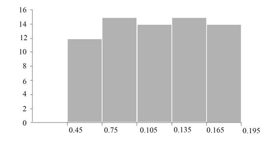
Figure 1

Interpretation:

Figure 1 represents the histogram for the given data.

Statistics Concept Introduction

A histogram is a bar graph of a frequency distribution of quantitative data.

Put classes along $x\text{-axis}$ and frequency along $y\text{-axis}$. Mark class mid- point of every class along $x\text{-axis}$. The width of each bar represents the width of each class. Width of each class should be same and each bar should touch each other.

(b)

To determine

To calculate:

The relative frequency for each class.

Answer to Problem 9E

Solution:

Required relative frequency table is,

Class	Relative Frequency
$0.05\text{-}0.07$	$17\%$
$0.08\text{-}0.10$	$21\%$
$0.11\text{-}0.13$	$20\%$
$0.14\text{-}0.16$	$21\%$
$0.17\text{-}0.19$	$20\%$

Explanation of Solution

Given information:

Braking Times for Vehicles at 60 mph (in Minutes)
Class	Frequency
$0.05\text{-}0.07$	12
$0.08\text{-}0.10$	15
$0.11\text{-}0.13$	14
$0.14\text{-}0.16$	15
$0.17\text{-}0.19$	14

Formula used:

Relative Frequency

$=\frac{f}{n}$

$\begin{array}{l}n=\text{sum}\text{of}\text{frequencies}\\ f=\text{frequency}\text{for}\text{the}\text{class}\end{array}$

Calculation:

Compute $n:$.

$\begin{array}{rll}n& =& 12+15+14+15+14\\ & =& 70\end{array}$

Compute relative frequencies for each class in the following table.

Class	Frequency	Relative Frequency
$0.05\text{-}0.07$	12	$\frac{f}{n}=\frac{12}{70}\approx 0.17=17\%$
$0.08\text{-}0.10$	15	$\frac{f}{n}=\frac{15}{70}\approx 0.21=21\%$
$0.11\text{-}0.13$	14	$\frac{f}{n}=\frac{14}{70}=0.2=20\%$
$0.14\text{-}0.16$	15	$\frac{f}{n}=\frac{15}{70}\approx 0.21=21\%$
$0.17\text{-}0.19$	14	$\frac{f}{n}=\frac{14}{70}=0.2=20\%$

Table 2

Conclusion:

Thus, the required relative frequency table is,

Class	Relative Frequency
$0.05\text{-}0.07$	$17\%$
$0.08\text{-}0.10$	$21\%$
$0.11\text{-}0.13$	$20\%$
$0.14\text{-}0.16$	$21\%$
$0.17\text{-}0.19$	$20\%$

(c)

To determine

To graph:

A relative frequency histogram for the given data.

Explanation of Solution

Given information:

Class	Frequency	Relative Frequency
$0.05\text{-}0.07$	12	$17\%$
$0.08\text{-}0.10$	15	$21\%$
$0.11\text{-}0.13$	14	$20\%$
$0.14\text{-}0.16$	15	$21\%$
$0.17\text{-}0.19$	14	$20\%$

Formula used:

Class mid-point $=\frac{\text{upper}\text{limit}\text{of}\text{class}+\text{lower}\text{limit}\text{of}\text{class}}{2}$

$p$$=\frac{\text{lower}\text{limit}\text{of}\text{succeding}\text{class}-\text{upper}\text{limit}\text{of}\text{the}\text{class}}{2}$

For adjustment of class boundaries subtract $p$ from lower limit and $p$ with upper limit of each class.

Calculation:

Compute the class mid-point of each class.

For the class $0.05\text{-}0.07$,

$\begin{array}{rcl}\text{Class mid‐point}& =& \frac{\text{upper\hspace{0.17em}limit\hspace{0.17em}of\hspace{0.17em}class}+\text{lower\hspace{0.17em}limit\hspace{0.17em}of\hspace{0.17em}class}}{2}\\ & =& \frac{0.05+0.07}{2}\\ & =& 0.06\end{array}$

For the class $0.08\text{-}0.10$,

$\begin{array}{rcl}\text{Class mid‐point}& =& \frac{\text{upper\hspace{0.17em}limit\hspace{0.17em}of\hspace{0.17em}class}+\text{lower\hspace{0.17em}limit\hspace{0.17em}of\hspace{0.17em}class}}{2}\\ & =& \frac{0.08+0.10}{2}\\ & =& 0.09\end{array}$

For the class $0.11\text{-}0.13$,

$\begin{array}{rcl}\text{Class mid‐point}& =& \frac{\text{upper\hspace{0.17em}limit\hspace{0.17em}of\hspace{0.17em}class}+\text{lower\hspace{0.17em}limit\hspace{0.17em}of\hspace{0.17em}class}}{2}\\ & =& \frac{0.11+0.13}{2}\\ & =& 0.12\end{array}$

For the class $0.14\text{-}0.16$,

$\begin{array}{rcl}\text{Class mid‐point}& =& \frac{\text{upper\hspace{0.17em}limit\hspace{0.17em}of\hspace{0.17em}class}+\text{lower\hspace{0.17em}limit\hspace{0.17em}of\hspace{0.17em}class}}{2}\\ & =& \frac{0.14+0.16}{2}\\ & =& 0.15\end{array}$

For the class $0.17\text{-}0.19$,

$\begin{array}{rcl}\text{Class mid‐point}& =& \frac{\text{upper\hspace{0.17em}limit\hspace{0.17em}of\hspace{0.17em}class}+\text{lower\hspace{0.17em}limit\hspace{0.17em}of\hspace{0.17em}class}}{2}\\ & =& \frac{0.17+0.19}{2}\\ & =& 0.18\end{array}$

Calculate the adjustment factor.

$\begin{array}{rcl}p& =& \frac{{\displaystyle 0.08-0.07}}{{\displaystyle 2}}\\ & =& \frac{{\displaystyle 0.01}}{{\displaystyle 2}}\\ & =& 0.005\end{array}\begin{array}{}\end{array}$

Construct the table with adjusted class boundary and class mid-point.

Braking Times for Vehicles at 60 mph (in Minutes)
Class boundary	Mid-point	Relative Frequency
$0.045\text{-}0.075$	0.06	$17\%$
$0.075\text{-}0.105$	0.09	$21\%$
$0.105\text{-}0.135$	0.12	$20\%$
$0.135\text{-}0.165$	0.15	$21\%$
$0.165\text{-}0.195$	0.18	$20\%$

Table 3

Graph:

Construct the relative frequency histogram corresponding to the table 3.

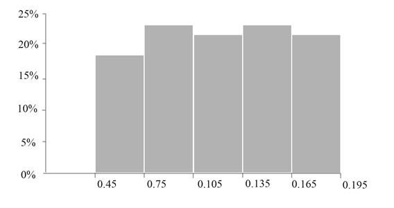
Figure 2

Interpretation:

Figure 2 represents the relative frequency histogram for the given data.

Statistics Concept Introduction

A histogram is a bar graph of a frequency distribution of quantitative data.

Put classes along $x\text{-axis}$ and relative frequency along $y\text{-axis}$. Mark class mid- point of every class along $x\text{-axis}$. The width of each bar represents the width of each class. Width of each class should be same and each bar should touch each other.