
Concept explainers
a.
To create: A scatter plot showing the deficit on horizontal axis and changes in and bond holding on vertical axis.
a.
Explanation of Solution
Table showing calculation of change in public bond holdings, Federal Reserve bond holding and changes in debt held by public and federal reserve is as follows:
| Period | Budget Deficit | debt held by public | debt held by federal reserve | change in debt held by public | change in debt held by federal reserve | changes in debt held by public and federal reserve |
| 1980-01-01 | 73830 | 699384 | 120800.0 | - | - | - |
| 1981-01-01 | 78968 | 790060 | 123575.0 | 90676 | 2775.0 | 93450.5 |
| 1982-01-01 | 127977 | 910039 | 131825.0 | 119979 | 8250.0 | 128228.8 |
| 1983-01-01 | 207802 | 1111561 | 146425.0 | 201522 | 14600.0 | 216122.3 |
| 1984-01-01 | 185367 | 1290387 | 154900.0 | 178826 | 8475.0 | 187301.0 |
| 1985-01-01 | 212308 | 1494839 | 170275.0 | 204453 | 15375.0 | 219827.5 |
| 1986-01-01 | 221227 | 1718347 | 192700.0 | 223508 | 22425.0 | 245932.5 |
| 1987-01-01 | 149730 | 1889399 | 210800.0 | 171052 | 18100.0 | 189152.3 |
| 1988-01-01 | 155178 | 2039260 | 228175.0 | 149861 | 17375.0 | 167235.8 |
| 1989-01-01 | 152639 | 2175360 | 227075.0 | 136100 | -1100.0 | 134999.8 |
| 1990-01-01 | 221036 | 2418033 | 229700.0 | 242674 | 2625.0 | 245298.5 |
| 1991-01-01 | 269238 | 2704994 | 253400.0 | 286961 | 23700.0 | 310661.3 |
| 1992-01-01 | 290321 | 3018001 | 279350.0 | 313007 | 25950.0 | 338956.5 |
| 1993-01-01 | 255051 | 3279209 | 315750.0 | 261208 | 36400.0 | 297607.8 |
| 1994-01-01 | 203186 | 3474962 | 350600.0 | 195753 | 34850.0 | 230603.0 |
| 1995-01-01 | 163952 | 3645419 | 370550.0 | 170457 | 19950.0 | 190407.3 |
| 1996-01-01 | 107431 | 3776614 | 383950.0 | 131195 | 13400.0 | 144594.8 |
| 1997-01-01 | 21884 | 3835440 | 412125.0 | 58827 | 28175.0 | 87001.8 |
| 1998-01-01 | 69270 | 3803038 | 442775.0 | -32403 | 30650.0 | -1752.5 |
| 1999-01-01 | 125610 | 3715711 | 479400.0 | -87327 | 36625.0 | -50701.8 |
| 2000-01-01 | 236241 | 3508911 | 507425.0 | -206800 | 28025.0 | -178775.0 |
| 2001-01-01 | 128236 | 3360257 | 536200.0 | -148654 | 28775.0 | -119879.3 |
| 2002-01-01 | 157758 | 3526798 | 599925.0 | 166541 | 63725.0 | 230266.0 |
| 2003-01-01 | 377585 | 3873789 | 654100.0 | 346992 | 54175.0 | 401166.5 |
| 2004-01-01 | 412727 | 4276280 | 694900.0 | 402491 | 40800.0 | 443290.5 |
| 2005-01-01 | 318346 | 4604003 | 730650.0 | 327723 | 35750.0 | 363473.3 |
| 2006-01-01 | 248181 | 4853668 | 768175.0 | 249665 | 37525.0 | 287189.5 |
| 2007-01-01 | 160701 | 5045710 | 772900.0 | 192043 | 4725.0 | 196767.8 |
| 2008-01-01 | 458553 | 5701491 | 505625.0 | 655781 | -267275.0 | 388505.8 |
| 2009-01-01 | 1412688 | 7345425 | 673650.0 | 1643934 | 168025.0 | 1811958.5 |
| 2010-01-01 | 1294373 | 8839123 | 846725.0 | 1493699 | 173075.0 | 1666773.8 |
| 2011-01-01 | 1299599 | 9996999 | 1572000.0 | 1157875 | 725275.0 | 1883150.3 |
| 2012-01-01 | 1086955 | 11196392 | 1658100.0 | 1199393 | 86100.0 | 1285493.3 |
| 2013-01-01 | 679542 | 12041300 | 2003425.0 | 844908 | 345325.0 | 1190233.0 |
| 2014-01-01 | 484600 | 12755962 | 2720300.0 | 714663 | 716875.0 | 1431537.5 |
| 2015-01-01 | 438496 | 13247211 | 2802050.0 | 491249 | 81750.0 | 572998.5 |
| 2016-01-01 | 584651 | 14121037 | 2827050.0 | 873826 | 25000.0 | 898826.0 |
| 2017-01-01 | 665372 | 14562572 | 2862225.0 | 441535 | 35175.0 | 476710.3 |
Table (1)
Scatter diagram showing public bond holding on the vertical axis and deficit on horizontal axis is as follows:
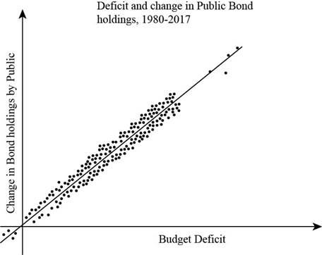
Fig.1
The steep fitted line in Fig. 1 shows the strong relation between the change in debt held by public and deficit from 1980-2017
Introduction:
When the planned expenditure of government exceeds the amount of revenue available to pay for it, it is known as budget deficit.
b.
To create: A scatter plot showing the deficit on horizontal axis and changes in and bond holding by Federal Reserve on vertical axis from 1980-2017.
b.
Explanation of Solution
Diagram showing Federal Reserve bond holdings on the vertical axis and deficit on horizontal axis since 1980 to 2017, is as follows:
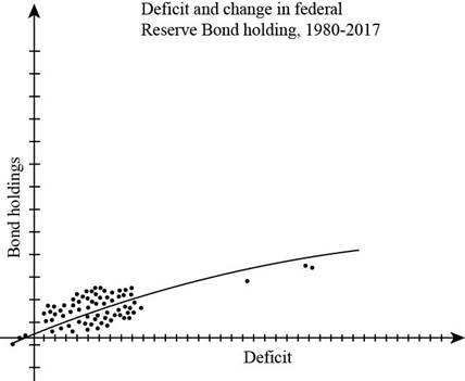
Fig.2
The steeper fitted line shows the positive relationship between bond holdings by the Federal Reserve and deficit but with less prognostic power.
Introduction:
When the planned expenditure of government exceeds the amount of revenue available to pay for it, it is known as budget deficit
c.
To create: A scatter plot showing the deficit on horizontal axis and changes in and bond holding by Federal Reserve on vertical axis from 1980-2007.
c.
Explanation of Solution
Diagram showing Federal Reserve bond holdings on the vertical axis and deficit on horizontal axis since 1980 to 2007, is as follows:
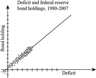
Fig.3
As the fitted line in Fig.1 suggests there was a positive relationship between bond holdings by the Federal Reserve and deficit from1980-2007.
Introduction:
When the planned expenditure of government exceeds the amount of revenue available to pay for it, it is known as budget deficit.
Want to see more full solutions like this?
Chapter 22 Solutions
EBK ECONOMICS OF MONEY, BANKING AND FIN


- 1. Repeated rounds of negotiation exacerbate the incentive to free-ride that exists for nations considering the ratification of international environmental agreements.arrow_forwardFor environmental Economics, A-C Pleasearrow_forwardTrue/ False/ Undetermined - Environmental Economics 3. When the MAC is known but there is uncertainty about the MDF, an emissions quota leads to a lower deadweight loss associated with this uncertainty.arrow_forward
- True/False/U- Environmental Economics 2. The discount rate used in climate integrated assessment models is the key driver of the intensity of emissions reductions associated with optimal climate policy in the model.arrow_forwardAt the beginning of the year, the market for portable electric fans was in equilibrium. In June, a summer heat wave hit. What effect does the heat wave have on the market for fans? Drag the appropriate part(s) of the graph to show the effect on the market for portable fans. To refer to the graphing tutorial for this question type, please click here. Price 17 OF 21 QUESTIONS COMPLETED f4 Q Search f5 f6 f7 CO hp fg 6 M366 W ins f12 f11 f10 SUBMIT ANSWER ENG 4xarrow_forwardIn the context of investment risk, what does "diversification" mean? A) Spreading investments across various assets to reduce riskB) Investing in a single asset to maximize returnsC) Increasing investment in high-risk assetsD) Reducing the number of investments to focus on high-performing onesarrow_forward
- At the 8:10 café, there are equal numbers of two types of customers with the following values. The café owner cannot distinguish between the two types of students because many students without early classes arrive early anyway (that is she cannot price discriminate). Students with early classes Students without early classes Coffee 70 60 Banana 50 100 The MC of coffee is 10. The MC of a banana is 40. Is bundling more profitable than selling separately? HINT: if you sell the bundle, can you make more by offering coffee separately? If so, what price should be charged for the bundle? (Show calculations)arrow_forwardYour marketing department has identified the following customer demographics in the following table. Construct a demand curve and determine the profit maximizing price as well as the expected profit if MC=$1. The number of customers in the target population is 10,000. Use the following demand data: Group Value Frequency Baby boomers $5 20% Generation X $4 10% Generation Y $3 10% `Tweeners $2 10% Seniors $2 10% Others $0 40%arrow_forwardYour marketing department has identified the following customer demographics in the following table. Construct a demand curve and determine the profit maximizing price as well as the expected profit if MC=$1. The number of customers in the target population is 10,000. Group Value Frequency Baby boomers $5 20% Generation X $4 10% Generation Y $3 10% `Tweeners $2 10% Seniors $2 10% Others $0 40% ur marketing department has identified the following customer demographics in the following table. Construct a demand curve and determine the profit maximizing price as well as the expected profit if MC=$1. The number of customers in the target population is 10,000.arrow_forward
- Test Preparation QUESTION 2 [20] 2.1 Body Mass Index (BMI) is a summary measure of relative health. It is calculated by dividing an individual's weight (in kilograms) by the square of their height (in meters). A small sample was drawn from the population of UWC students to determine the effect of exercise on BMI score. Given the following table, find the constant and slope parameters of the sample regression function of BMI = f(Weekly exercise hours). Interpret the two estimated parameter values. X (Weekly exercise hours) Y (Body-Mass index) QUESTION 3 2 4 6 8 10 12 41 38 33 27 23 19 Derek investigates the relationship between the days (per year) absent from work (ABSENT) and the number of years taken for the worker to be promoted (PROMOTION). He interviewed a sample of 22 employees in Cape Town to obtain information on ABSENT (X) and PROMOTION (Y), and derived the following: ΣΧ ΣΥ 341 ΣΧΥ 176 ΣΧ 1187 1012 3.1 By using the OLS method, prove that the constant and slope parameters of the…arrow_forwardQUESTION 2 2.1 [30] Mariana, a researcher at the World Health Organisation (WHO), collects information on weekly study hours (HOURS) and blood pressure level when writing a test (BLOOD) from a sample of university students across the country, before running the regression BLOOD = f(STUDY). She collects data from 5 students as listed below: X (STUDY) 2 Y (BLOOD) 4 6 8 10 141 138 133 127 123 2.1.1 By using the OLS method and the information above derive the values for parameters B1 and B2. 2.1.2 Derive the RSS (sum of squares for the residuals). 2.1.3 Hence, calculate ô 2.2 2.3 (6) (3) Further, she replicates her study and collects data from 122 students from a rival university. She derives the residuals followed by computing skewness (S) equals -1.25 and kurtosis (K) equals 8.25 for the rival university data. Conduct the Jacque-Bera test of normality at a = 0.05. (5) Upon tasked with deriving estimates of ẞ1, B2, 82 and the standard errors (SE) of ẞ1 and B₂ for the replicated data.…arrow_forwardIf you were put in charge of ensuring that the mining industry in canada becomes more sustainable over the course of the next decade (2025-2035), how would you approach this? Come up with (at least) one resolution for each of the 4 major types of conflict: social, environmental, economic, and politicalarrow_forward

 Principles of Economics (12th Edition)EconomicsISBN:9780134078779Author:Karl E. Case, Ray C. Fair, Sharon E. OsterPublisher:PEARSON
 Engineering Economy (17th Edition)EconomicsISBN:9780134870069Author:William G. Sullivan, Elin M. Wicks, C. Patrick KoellingPublisher:PEARSON
 Principles of Economics (MindTap Course List)EconomicsISBN:9781305585126Author:N. Gregory MankiwPublisher:Cengage Learning
 Managerial Economics: A Problem Solving ApproachEconomicsISBN:9781337106665Author:Luke M. Froeb, Brian T. McCann, Michael R. Ward, Mike ShorPublisher:Cengage Learning
 Managerial Economics & Business Strategy (Mcgraw-...EconomicsISBN:9781259290619Author:Michael Baye, Jeff PrincePublisher:McGraw-Hill Education