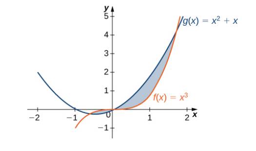
For the following exercises, split the region between the two curves into two smaller regions, then determine the area by integrating over the x-axis. Note that you will have two
3.

Trending nowThis is a popular solution!

Chapter 2 Solutions
Calculus Volume 2
Additional Math Textbook Solutions
Elementary Statistics: Picturing the World (7th Edition)
University Calculus: Early Transcendentals (4th Edition)
Using and Understanding Mathematics: A Quantitative Reasoning Approach (6th Edition)
Calculus: Early Transcendentals (2nd Edition)
Elementary Statistics (13th Edition)
Graphical Approach To College Algebra
- If -1 "[a446]-[254] 4b = -1 , find the values of a and b. ○ There is no solution for a and b. ○ There are infinite solutions for a and b. O a=3, b=3 O a=1, b=2 O a=2, b=1 O a=2, b=2arrow_forwardA student puts a 3x3 system of linear equations is into an augmented matrix. The student then correctly puts the augmented matrix into row echelon form (REF), which yields the following resultant matrix: -2 3 -0.5 10 0 0 0 -2 0 1 -4 Which of the following conclusions is mathematically supported by the work shown about system of linear equations? The 3x3 system of linear equations has no solution. ○ The 3x3 system of linear equations has infinite solutions. The 3x3 system of linear equations has one unique solution.arrow_forwardSolve the following system of equations using matrices: -2x + 4y = 8 and 4x - 3y = 9 Note: This is the same system of equations referenced in Question 14. If a single solution exists, express your solution as an (x,y) coordinate point with no spaces. If there are infinite solutions write inf and if there are no solutions write ns in the box.arrow_forward
- Hi, I need to make sure I have drafted a thorough analysis, so please answer the following questions. Based on the data in the attached image, develop a regression model to forecast the average sales of football magazines for each of the seven home games in the upcoming season (Year 10). That is, you should construct a single regression model and use it to estimate the average demand for the seven home games in Year 10. In addition to the variables provided, you may create new variables based on these variables or based on observations of your analysis. Be sure to provide a thorough analysis of your final model (residual diagnostics) and provide assessments of its accuracy. What insights are available based on your regression model?arrow_forwardI want to make sure that I included all possible variables and observations. There is a considerable amount of data in the images below, but not all of it may be useful for your purposes. Are there variables contained in the file that you would exclude from a forecast model to determine football magazine sales in Year 10? If so, why? Are there particular observations of football magazine sales from previous years that you would exclude from your forecasting model? If so, why?arrow_forwardStat questionsarrow_forward
- 1) and let Xt is stochastic process with WSS and Rxlt t+t) 1) E (X5) = \ 1 2 Show that E (X5 = X 3 = 2 (= = =) Since X is WSSEL 2 3) find E(X5+ X3)² 4) sind E(X5+X2) J=1 ***arrow_forwardQuestion 1: Let X be a random variable with p.m.f (|x| +1)² x= -2, -1, 0, 1,2 f(x) = C 0, O.W 1. The value of c. 2. The c.d.f. 3. E(X). 4. E(2x+3). 5. E(X²). 6. E(3x²+4). 7. E(X(3X+4)). 8. Var(X). 9. Var (6-3X). 10. Find the m.g.f of the random variable Xarrow_forwardI need help explaining on this examplearrow_forward
- Prove that 1) | RxX (T) | << = (R₁ " + R$) 2) find Laplalse trans. of Normal dis: 3) Prove thy t /Rx (z) | < | Rx (0)\ 4) show that evary algebra is algebra or not.arrow_forward= 5 37 A 4 8 0.5 06 9arrow_forwardFor each of the time series, construct a line chart of the data and identify the characteristics of the time series (that is, random, stationary, trend, seasonal, or cyclical). Month Number (Thousands)Dec 1991 65.60Jan 1992 71.60Feb 1992 78.80Mar 1992 111.60Apr 1992 107.60May 1992 115.20Jun 1992 117.80Jul 1992 106.20Aug 1992 109.90Sep 1992 106.00Oct 1992 111.80Nov 1992 84.50Dec 1992 78.60Jan 1993 70.50Feb 1993 74.60Mar 1993 95.50Apr 1993 117.80May 1993 120.90Jun 1993 128.50Jul 1993 115.30Aug 1993 121.80Sep 1993 118.50Oct 1993 123.30Nov 1993 102.30Dec 1993 98.70Jan 1994 76.20Feb 1994 83.50Mar 1994 134.30Apr 1994 137.60May 1994 148.80Jun 1994 136.40Jul 1994 127.80Aug 1994 139.80Sep 1994 130.10Oct 1994 130.60Nov 1994 113.40Dec 1994 98.50Jan 1995 84.50Feb 1995 81.60Mar 1995 103.80Apr 1995 116.90May 1995 130.50Jun 1995 123.40Jul 1995 129.10Aug 1995…arrow_forward
 Elementary Geometry For College Students, 7eGeometryISBN:9781337614085Author:Alexander, Daniel C.; Koeberlein, Geralyn M.Publisher:Cengage,
