
Concept explainers
Videos
Decimal Data: Batting Averages The following data represent baseball batting averages for a random sample of National League players neat the end of the baseball season. the data are from the baseball statistics section of the Denver Post.
| 0.194 | 0.258 | 0.190 | 0.291 | 0.158 | 0.295 | 0.261 | 0.250 | 0.181 |
| 0.125 | 0.107 | 0.260 | 0.309 | 0.309 | 0.276 | 0.287 | 0.317 | 0.252 |
| 0.215 | 0.250 | 0.246 | 0.260 | 0.265 | 0.182 | 0.113 | 0.200 |
(a) Multiply each data value by 1000 to “clear” the decimals.
(b) Use the standard procedares of this section to make a frequency table and histogram with your whole-number data. Use five classes.
(c) Divide class limits, class boundaries, and class midpoints by 1000 to get back to your original dat.
(a)
To find: The decimal data that are multiply with 1000 for each value in the data..
Answer to Problem 22P
Solution: The data multiply with 1000 for each value in the data is as follows:
| Data | Data*100 | Data | Data*100 |
| 0.194 | 194 | 0.309 | 309 |
| 0.258 | 258 | 0.276 | 276 |
| 0.19 | 190 | 0.287 | 287 |
| 0.291 | 291 | 0.317 | 317 |
| 0.158 | 158 | 0.252 | 252 |
| 0.295 | 295 | 0.215 | 215 |
| 0.261 | 261 | 0.25 | 250 |
| 0.25 | 250 | 0.246 | 246 |
| 0.181 | 181 | 0.26 | 260 |
| 0.125 | 125 | 0.265 | 265 |
| 0.107 | 107 | 0.182 | 182 |
| 0.26 | 260 | 0.113 | 113 |
| 0.309 | 309 | 0.2 | 200 |
Explanation of Solution
Calculation: The data represent baseball batting averages for a random sample of National League players near the end of the baseball season and there are 26 values in the data set. To find the whole number data by multiplying 1000 is obtained as follows:
| Data | Data*100 | Data | Data*100 |
| 0.194 | 0.309 | 309 | |
| 0.258 | 0.276 | 276 | |
| 0.19 | 0.287 | 287 | |
| 0.291 | 291 | 0.317 | 317 |
| 0.158 | 158 | 0.252 | 252 |
| 0.295 | 295 | 0.215 | 215 |
| 0.261 | 261 | 0.25 | 250 |
| 0.25 | 250 | 0.246 | 246 |
| 0.181 | 181 | 0.26 | 260 |
| 0.125 | 125 | 0.265 | 265 |
| 0.107 | 107 | 0.182 | 182 |
| 0.26 | 260 | 0.113 | 113 |
| 0.309 | 309 | 0.2 | 200 |
Interpretation: Hence, the data multiply with 1000 is as follows:
| Data | Data*100 | Data | Data*100 |
| 0.194 | 194 | 0.309 | 309 |
| 0.258 | 258 | 0.276 | 276 |
| 0.19 | 190 | 0.287 | 287 |
| 0.291 | 291 | 0.317 | 317 |
| 0.158 | 158 | 0.252 | 252 |
| 0.295 | 295 | 0.215 | 215 |
| 0.261 | 261 | 0.25 | 250 |
| 0.25 | 250 | 0.246 | 246 |
| 0.181 | 181 | 0.26 | 260 |
| 0.125 | 125 | 0.265 | 265 |
| 0.107 | 107 | 0.182 | 182 |
| 0.26 | 260 | 0.113 | 113 |
| 0.309 | 309 | 0.2 | 200 |
(b)
To find: The standard frequency table for the data set..
Answer to Problem 22P
Solution: The complete frequency table is as:
| Class limits | Class boundaries | Midpoints | Freq | Relative freq | Cumulative freq |
| 46-85 | 45.5-85.5 | 65.5 | 4 | 0.12 | 4 |
| 86-125 | 85.5-125.5 | 105.5 | 5 | 0.16 | 9 |
| 126-165 | 125.5-165.5 | 145.5 | 10 | 0.31 | 19 |
| 166-205 | 165.5-205.5 | 185.5 | 5 | 0.16 | 24 |
| 206-245 | 205.5-245.5 | 225.5 | 5 | 0.16 | 29 |
| 246-285 | 245.5-285.5 | 265.5 | 3 | 0.09 | 32 |
Explanation of Solution
Calculation: To find the class width for the whole data of 26 values, it is observed that largest value of the data set is 317 and the smallest value is 107 in the data. Using 5 classes, the class width calculated in the following way:
The value is round up to the nearest whole number. Hence, the class width of the data set is 43. The class width for the data is 43 and the lowest data value (107) will be the lower class limit of the first class. Because the class width is 43, it must add 43 to the lowest class limit in the first class to find the lowest class limit in the second class. There are 5 desired classes. Hence, the class limits are 107–149, 150–192, 193–235, 236–278, and 279–321. Now, to find the class boundaries subtract 0.5 from lower limit of every class and add 0.5 to the upper limit of the every class interval. Hence, the class boundaries are 106.5–149.5, 149.5–192.5, 192.5–235.5, 235.5-278.5, and 278.5-321.5.
Next to find the midpoint of the class is calculated by using formula,
Midpoint of first class is calculated as:
The frequencies for respective classes are 3, 4, 3, 10, and 6.
Relative frequency is calculated by using the formula
The frequency for first class is 3 and total frequencies are 26 so the relative frequency is
The calculated frequency table is as follows:
| Class limits | Class boundaries | Midpoints | freq | relative freq |
| 107-149 | 106.5-149.5 | 128 | 3 | 0.12 |
| 150-192 | 149.5-192.5 | 171 | 4 | 0.15 |
| 193-235 | 192.5-235.5 | 214 | 3 | 0.12 |
| 236-278 | 235.5-278.5 | 257 | 10 | 0.38 |
| 279-321 | 278.5-321.5 | 300 | 6 | 0.23 |
Graph: To construct the histogram by using the MINITAB, the steps are as follows:
Step 1: Enter the class boundaries in C1 and frequency in C2.
Step 2: Go to Graph > Histogram > Simple.
Step 3: Enter C1 in Graph variable then go to Data options > Frequency > C2.
Step 4: Click on OK.
The obtained histogram is
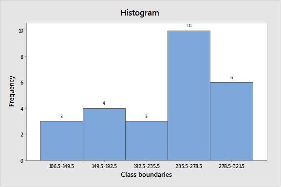
Interpretation: Hence, the complete frequency table is as follows:
| Class limits | Class boundaries | Midpoints | Freq | Relative freq |
| 107-149 | 106.5-149.5 | 128 | 3 | 0.12 |
| 150-192 | 149.5-192.5 | 171 | 4 | 0.15 |
| 193-235 | 192.5-235.5 | 214 | 3 | 0.12 |
| 236-278 | 235.5-278.5 | 257 | 10 | 0.38 |
| 279-321 | 278.5-321.5 | 300 | 6 | 0.23 |
(c)
To find: The class limits, class boundaries, and midpoints in the frequency table by dividing 1000..
Answer to Problem 22P
Solution: The frequency table of original data is as follows:
| Class limits | Class boundaries | Midpoints | |
| 0.107-0.149 | 0.1065-0.1495 | 0.128 | |
| 0.149-0.192 | 0.1495-0.1925 | 0.171 | |
| 0.193-0.235 | 0.1925-0.2355 | 0.214 | |
| 0.236-0.278 | 0.2355-0.2785 | 0.257 | |
| 0.279-0.321 | 0.2785-0.3215 | 0.3 | |
Explanation of Solution
Calculation: The frequency table for whole number is obtained in above part. It is the data that multiply each value by 1000 to ‘clear’ decimals from the data. The frequency table for whole number is as follows:
| Class limits | Class boundaries | Midpoints | Freq | Relative freq |
| 107–149 | 106.5–149.5 | 128 | 3 | 0.12 |
| 150–192 | 149.5–192.5 | 171 | 4 | 0.15 |
| 193–235 | 192.5–235.5 | 214 | 3 | 0.12 |
| 236–278 | 235.5–278.5 | 257 | 10 | 0.38 |
| 279–321 | 278.5–321.5 | 300 | 6 | 0.23 |
To find the decimal or original data, divide the class limits, class boundaries, and midpoints by 1000. The calculation as follows:
| Class limits | Class boundaries | Midpoints | |
| 0.107–0.149 | 0.1065–0.1495 | 0.128 | |
| 0.149–0.192 | 0.1495–0.1925 | 0.171 | |
| 0.193–0.235 | 0.1925–0.2355 | 0.214 | |
| 0.236–0.278 | 0.2355–0.2785 | 0.257 | |
| 0.279–0.321 | 0.2785–0.3215 | 0.3 | |
Interpretation: Hence, the data divide by 1000 is as follows:
| Class limits | Class boundaries | Midpoints | |
| 0.107–0.149 | 0.1065–0.1495 | 0.128 | |
| 0.149–0.192 | 0.1495–0.1925 | 0.171 | |
| 0.193–0.235 | 0.1925–0.2355 | 0.214 | |
| 0.236–0.278 | 0.2355–0.2785 | 0.257 | |
| 0.279–0.321 | 0.2785–0.3215 | 0.300 | |
Want to see more full solutions like this?
Chapter 2 Solutions
Understanding Basic Statistics


- Harvard University California Institute of Technology Massachusetts Institute of Technology Stanford University Princeton University University of Cambridge University of Oxford University of California, Berkeley Imperial College London Yale University University of California, Los Angeles University of Chicago Johns Hopkins University Cornell University ETH Zurich University of Michigan University of Toronto Columbia University University of Pennsylvania Carnegie Mellon University University of Hong Kong University College London University of Washington Duke University Northwestern University University of Tokyo Georgia Institute of Technology Pohang University of Science and Technology University of California, Santa Barbara University of British Columbia University of North Carolina at Chapel Hill University of California, San Diego University of Illinois at Urbana-Champaign National University of Singapore McGill…arrow_forwardName Harvard University California Institute of Technology Massachusetts Institute of Technology Stanford University Princeton University University of Cambridge University of Oxford University of California, Berkeley Imperial College London Yale University University of California, Los Angeles University of Chicago Johns Hopkins University Cornell University ETH Zurich University of Michigan University of Toronto Columbia University University of Pennsylvania Carnegie Mellon University University of Hong Kong University College London University of Washington Duke University Northwestern University University of Tokyo Georgia Institute of Technology Pohang University of Science and Technology University of California, Santa Barbara University of British Columbia University of North Carolina at Chapel Hill University of California, San Diego University of Illinois at Urbana-Champaign National University of Singapore…arrow_forwardA company found that the daily sales revenue of its flagship product follows a normal distribution with a mean of $4500 and a standard deviation of $450. The company defines a "high-sales day" that is, any day with sales exceeding $4800. please provide a step by step on how to get the answers in excel Q: What percentage of days can the company expect to have "high-sales days" or sales greater than $4800? Q: What is the sales revenue threshold for the bottom 10% of days? (please note that 10% refers to the probability/area under bell curve towards the lower tail of bell curve) Provide answers in the yellow cellsarrow_forward
- Find the critical value for a left-tailed test using the F distribution with a 0.025, degrees of freedom in the numerator=12, and degrees of freedom in the denominator = 50. A portion of the table of critical values of the F-distribution is provided. Click the icon to view the partial table of critical values of the F-distribution. What is the critical value? (Round to two decimal places as needed.)arrow_forwardA retail store manager claims that the average daily sales of the store are $1,500. You aim to test whether the actual average daily sales differ significantly from this claimed value. You can provide your answer by inserting a text box and the answer must include: Null hypothesis, Alternative hypothesis, Show answer (output table/summary table), and Conclusion based on the P value. Showing the calculation is a must. If calculation is missing,so please provide a step by step on the answers Numerical answers in the yellow cellsarrow_forwardShow all workarrow_forward
 Big Ideas Math A Bridge To Success Algebra 1: Stu...AlgebraISBN:9781680331141Author:HOUGHTON MIFFLIN HARCOURTPublisher:Houghton Mifflin Harcourt
 Glencoe Algebra 1, Student Edition, 9780079039897...AlgebraISBN:9780079039897Author:CarterPublisher:McGraw Hill
 Holt Mcdougal Larson Pre-algebra: Student Edition...AlgebraISBN:9780547587776Author:HOLT MCDOUGALPublisher:HOLT MCDOUGAL