
Videos
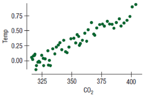
Climate change 2016 Data collected from around the globe (including the sea ice data of Exercise 23) show that the earth is getting warmer. The generally accepted explanation relates climate change to an increase in atmospheric levels of carbon dioxide (CO2) because CO2 is a greenhouse gas that traps the heat of the sun. A standard source of the mean annual CO2 concentration in the atmosphere (parts per million) is measurements taken at the top of Mauna Loa in Hawaii (away from any local contaminants) and available at ftp://aftp.cmdl.noaa.gov/ products/trends/co2/co2_annmean_mlo.txt.
Global temperature anomaly is the difference in mean global temperature relative to a base period of 1981 to 2010 in °C. It is available at www.ncdc.noaa.gov/cag/data-info/global.
Here are a
Response variable is: Temp
R squared = 89.7%
s = 0.0885 with 58 – 2 = 56 degrees of freedom
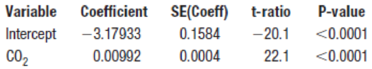
- a) Write the equation of the regression line.
- b) Is there evidence of an association between CO2 level and global temperature?
- c) Do you think predictions made by this regression will be very accurate? Explain.
- d) Does this regression prove that increasing CO2 levels are causing global warming? Discuss.
Want to see the full answer?
Check out a sample textbook solution
Chapter 20 Solutions
Intro Stats, Books a la Carte Edition (5th Edition)


- I need help with this problem and an explanation of the solution for the image described below. (Statistics: Engineering Probabilities)arrow_forward310015 K Question 9, 5.2.28-T Part 1 of 4 HW Score: 85.96%, 49 of 57 points Points: 1 Save of 6 Based on a poll, among adults who regret getting tattoos, 28% say that they were too young when they got their tattoos. Assume that six adults who regret getting tattoos are randomly selected, and find the indicated probability. Complete parts (a) through (d) below. a. Find the probability that none of the selected adults say that they were too young to get tattoos. 0.0520 (Round to four decimal places as needed.) Clear all Final check Feb 7 12:47 US Oarrow_forwardhow could the bar graph have been organized differently to make it easier to compare opinion changes within political partiesarrow_forward
- 30. An individual who has automobile insurance from a certain company is randomly selected. Let Y be the num- ber of moving violations for which the individual was cited during the last 3 years. The pmf of Y isy | 1 2 4 8 16p(y) | .05 .10 .35 .40 .10 a.Compute E(Y).b. Suppose an individual with Y violations incurs a surcharge of $100Y^2. Calculate the expected amount of the surcharge.arrow_forward24. An insurance company offers its policyholders a num- ber of different premium payment options. For a ran- domly selected policyholder, let X = the number of months between successive payments. The cdf of X is as follows: F(x)=0.00 : x < 10.30 : 1≤x<30.40 : 3≤ x < 40.45 : 4≤ x <60.60 : 6≤ x < 121.00 : 12≤ x a. What is the pmf of X?b. Using just the cdf, compute P(3≤ X ≤6) and P(4≤ X).arrow_forward59. At a certain gas station, 40% of the customers use regular gas (A1), 35% use plus gas (A2), and 25% use premium (A3). Of those customers using regular gas, only 30% fill their tanks (event B). Of those customers using plus, 60% fill their tanks, whereas of those using premium, 50% fill their tanks.a. What is the probability that the next customer will request plus gas and fill the tank (A2 B)?b. What is the probability that the next customer fills the tank?c. If the next customer fills the tank, what is the probability that regular gas is requested? Plus? Premium?arrow_forward
- 38. Possible values of X, the number of components in a system submitted for repair that must be replaced, are 1, 2, 3, and 4 with corresponding probabilities .15, .35, .35, and .15, respectively. a. Calculate E(X) and then E(5 - X).b. Would the repair facility be better off charging a flat fee of $75 or else the amount $[150/(5 - X)]? [Note: It is not generally true that E(c/Y) = c/E(Y).]arrow_forward74. The proportions of blood phenotypes in the U.S. popula- tion are as follows:A B AB O .40 .11 .04 .45 Assuming that the phenotypes of two randomly selected individuals are independent of one another, what is the probability that both phenotypes are O? What is the probability that the phenotypes of two randomly selected individuals match?arrow_forward53. A certain shop repairs both audio and video compo- nents. Let A denote the event that the next component brought in for repair is an audio component, and let B be the event that the next component is a compact disc player (so the event B is contained in A). Suppose that P(A) = .6 and P(B) = .05. What is P(BA)?arrow_forward

 Glencoe Algebra 1, Student Edition, 9780079039897...AlgebraISBN:9780079039897Author:CarterPublisher:McGraw Hill
 Algebra & Trigonometry with Analytic GeometryAlgebraISBN:9781133382119Author:SwokowskiPublisher:Cengage
 Big Ideas Math A Bridge To Success Algebra 1: Stu...AlgebraISBN:9781680331141Author:HOUGHTON MIFFLIN HARCOURTPublisher:Houghton Mifflin Harcourt