Concept explainers
Videos
Approximately 1.5 million high school students take the SAT each year and nearly 80% of the college and universities without open admissions policies use SAT scores in making admission decisions (College Board, March 2009). The current version of the SAT includes three parts: reading comprehension, mathematics, and writing. A perfect combined score for all three parts is 2400. A sample of SAT scores for the combined three-part SAT are as follows:
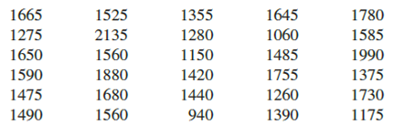
- a. Show a frequency distribution and histogram. Begin with the first class starting at 800 and use a class width of 200.
- b. Comment on the shape of the distribution.
- c. What other observations can be made about the SAT scores based on the tabular and graphical summaries?
a.
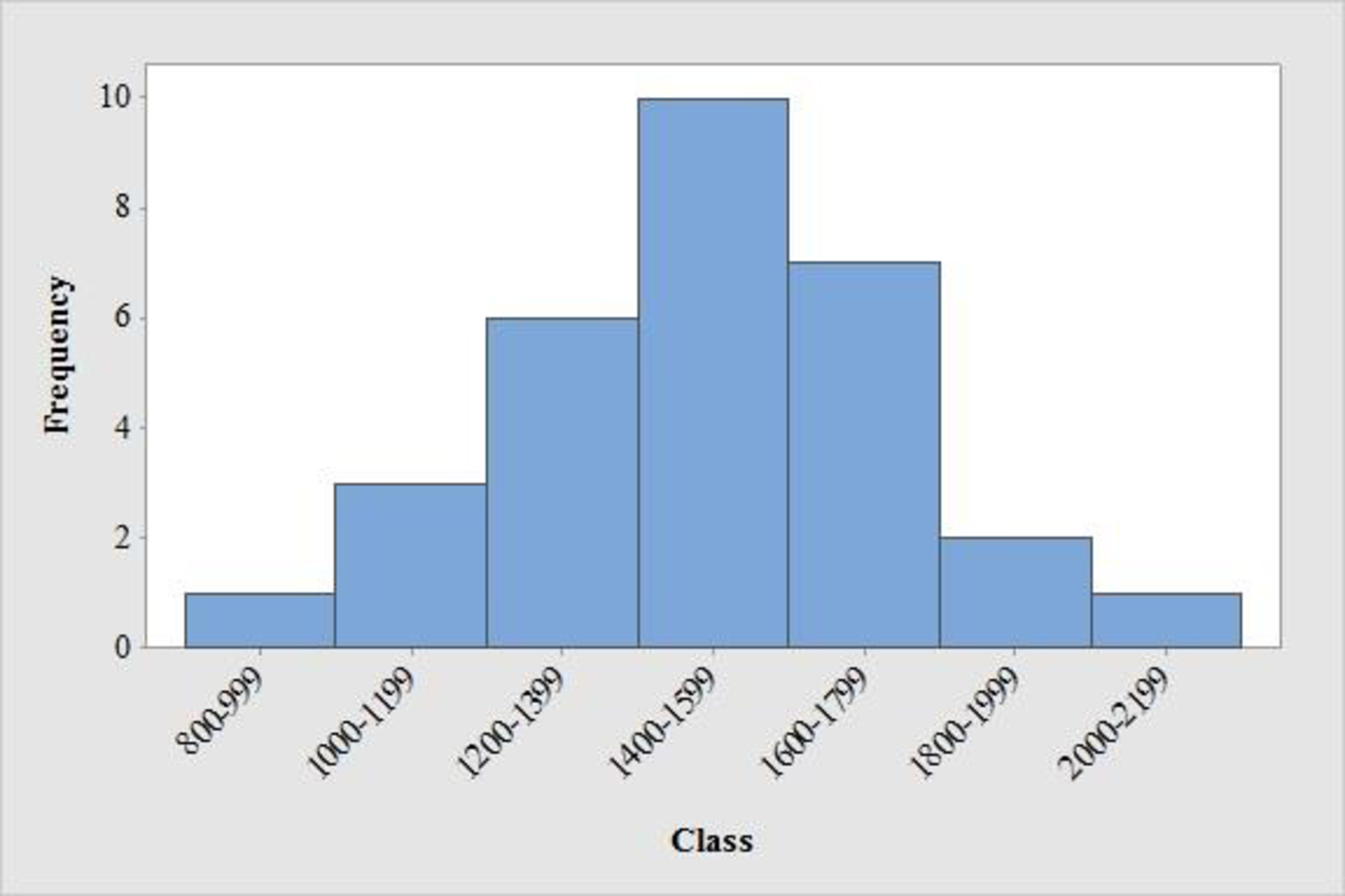
Construct the frequency distribution and histogram for the data.
Answer to Problem 44SE
The frequency distribution is tabulated below:
| Class | Tally | Frequency |
| 800-999 | 1 | |
| 1000-1199 | 3 | |
| 1200-1399 | 6 | |
| 1400-1599 | 10 | |
| 1600-1799 | 7 | |
| 1800-1999 | 2 | |
| 2000-2199 | 1 | |
| Total | 30 |
- Output using MINITAB software is given below:
Explanation of Solution
Calculation:
The data represents the sample of SAT scores for combined three part sat scores.
The frequencies are calculated by using the tally mark and the method of grouping is used because, range of the data is from 800 to 2,199. Here, the number of times each class levels repeats is the frequency of that particular class.
- From the given data set it is given that the class should be from approximately started with the class of 800 with class width of about 200.
- Make a tally mark for each value in the corresponding class and continue for all values in the data.
- The number of tally marks in each class represents the frequency, f of that class.
Similarly, the frequency of remaining classes for the data set is given below:
| Class | Tally | Frequency |
| 800-999 | 1 | |
| 1000-1199 | 3 | |
| 1200-1399 | 6 | |
| 1400-1599 | 10 | |
| 1600-1799 | 7 | |
| 1800-1999 | 2 | |
| 2000-2199 | 1 | |
| Total | 30 |
Software procedure:
Step by step procedure to draw the frequency histogram chart by using MINITAB software.
- Choose Graph > Histogram.
- Choose Simple, and then click OK.
- In Graph variables, enter the corresponding column of data.
- In scale on y-axis, make click on frequency.
- Click on ok.
b.
Comment the shape of the distribution.
Answer to Problem 44SE
The distribution of sat score is approximately symmetric.
Explanation of Solution
Symmetric distribution:
When the left and right sides of the distribution are approximately equal or mirror images of each other and three distributions will fall under symmetric distribution that is bell shaped, triangular and uniform or rectangular and then it is symmetric distribution.
From the graph, it is observed that the left and right side of the histogram is approximately equal. Hence, the shape of the distribution is bell-shaped curve.
Thus, it can be concluded that the distribution is approximately symmetric.
c.
Comment the observations of sat scores based on the tabular and graphical summary.
Explanation of Solution
From the data and the histogram, it is observed that approximately 33 percent of sat score (frequency about 10 of 30) will lie between 1400 and 1599.
- Moreover, the score less than 800 or greater than 2,200 are unusual and the average value of sat scores is over 1,500.
Want to see more full solutions like this?
Chapter 2 Solutions
STATISTICS F/BUSINESS+ECONOMICS-TEXT


- The PDF of an amplitude X of a Gaussian signal x(t) is given by:arrow_forwardThe PDF of a random variable X is given by the equation in the picture.arrow_forwardFor a binary asymmetric channel with Py|X(0|1) = 0.1 and Py|X(1|0) = 0.2; PX(0) = 0.4 isthe probability of a bit of “0” being transmitted. X is the transmitted digit, and Y is the received digit.a. Find the values of Py(0) and Py(1).b. What is the probability that only 0s will be received for a sequence of 10 digits transmitted?c. What is the probability that 8 1s and 2 0s will be received for the same sequence of 10 digits?d. What is the probability that at least 5 0s will be received for the same sequence of 10 digits?arrow_forward
- V2 360 Step down + I₁ = I2 10KVA 120V 10KVA 1₂ = 360-120 or 2nd Ratio's V₂ m 120 Ratio= 360 √2 H I2 I, + I2 120arrow_forwardQ2. [20 points] An amplitude X of a Gaussian signal x(t) has a mean value of 2 and an RMS value of √(10), i.e. square root of 10. Determine the PDF of x(t).arrow_forwardIn a network with 12 links, one of the links has failed. The failed link is randomlylocated. An electrical engineer tests the links one by one until the failed link is found.a. What is the probability that the engineer will find the failed link in the first test?b. What is the probability that the engineer will find the failed link in five tests?Note: You should assume that for Part b, the five tests are done consecutively.arrow_forward
- Problem 3. Pricing a multi-stock option the Margrabe formula The purpose of this problem is to price a swap option in a 2-stock model, similarly as what we did in the example in the lectures. We consider a two-dimensional Brownian motion given by W₁ = (W(¹), W(2)) on a probability space (Q, F,P). Two stock prices are modeled by the following equations: dX = dY₁ = X₁ (rdt+ rdt+0₁dW!) (²)), Y₁ (rdt+dW+0zdW!"), with Xo xo and Yo =yo. This corresponds to the multi-stock model studied in class, but with notation (X+, Y₁) instead of (S(1), S(2)). Given the model above, the measure P is already the risk-neutral measure (Both stocks have rate of return r). We write σ = 0₁+0%. We consider a swap option, which gives you the right, at time T, to exchange one share of X for one share of Y. That is, the option has payoff F=(Yr-XT). (a) We first assume that r = 0 (for questions (a)-(f)). Write an explicit expression for the process Xt. Reminder before proceeding to question (b): Girsanov's theorem…arrow_forwardProblem 1. Multi-stock model We consider a 2-stock model similar to the one studied in class. Namely, we consider = S(1) S(2) = S(¹) exp (σ1B(1) + (M1 - 0/1 ) S(²) exp (02B(2) + (H₂- M2 where (B(¹) ) +20 and (B(2) ) +≥o are two Brownian motions, with t≥0 Cov (B(¹), B(2)) = p min{t, s}. " The purpose of this problem is to prove that there indeed exists a 2-dimensional Brownian motion (W+)+20 (W(1), W(2))+20 such that = S(1) S(2) = = S(¹) exp (011W(¹) + (μ₁ - 01/1) t) 롱) S(²) exp (021W (1) + 022W(2) + (112 - 03/01/12) t). where σ11, 21, 22 are constants to be determined (as functions of σ1, σ2, p). Hint: The constants will follow the formulas developed in the lectures. (a) To show existence of (Ŵ+), first write the expression for both W. (¹) and W (2) functions of (B(1), B(²)). as (b) Using the formulas obtained in (a), show that the process (WA) is actually a 2- dimensional standard Brownian motion (i.e. show that each component is normal, with mean 0, variance t, and that their…arrow_forwardThe scores of 8 students on the midterm exam and final exam were as follows. Student Midterm Final Anderson 98 89 Bailey 88 74 Cruz 87 97 DeSana 85 79 Erickson 85 94 Francis 83 71 Gray 74 98 Harris 70 91 Find the value of the (Spearman's) rank correlation coefficient test statistic that would be used to test the claim of no correlation between midterm score and final exam score. Round your answer to 3 places after the decimal point, if necessary. Test statistic: rs =arrow_forward
- Business discussarrow_forwardBusiness discussarrow_forwardI just need to know why this is wrong below: What is the test statistic W? W=5 (incorrect) and What is the p-value of this test? (p-value < 0.001-- incorrect) Use the Wilcoxon signed rank test to test the hypothesis that the median number of pages in the statistics books in the library from which the sample was taken is 400. A sample of 12 statistics books have the following numbers of pages pages 127 217 486 132 397 297 396 327 292 256 358 272 What is the sum of the negative ranks (W-)? 75 What is the sum of the positive ranks (W+)? 5What type of test is this? two tailedWhat is the test statistic W? 5 These are the critical values for a 1-tailed Wilcoxon Signed Rank test for n=12 Alpha Level 0.001 0.005 0.01 0.025 0.05 0.1 0.2 Critical Value 75 70 68 64 60 56 50 What is the p-value for this test? p-value < 0.001arrow_forward
 Holt Mcdougal Larson Pre-algebra: Student Edition...AlgebraISBN:9780547587776Author:HOLT MCDOUGALPublisher:HOLT MCDOUGAL
 College Algebra (MindTap Course List)AlgebraISBN:9781305652231Author:R. David Gustafson, Jeff HughesPublisher:Cengage Learning
 Glencoe Algebra 1, Student Edition, 9780079039897...AlgebraISBN:9780079039897Author:CarterPublisher:McGraw Hill
 Big Ideas Math A Bridge To Success Algebra 1: Stu...AlgebraISBN:9781680331141Author:HOUGHTON MIFFLIN HARCOURTPublisher:Houghton Mifflin Harcourt