
Videos
Three groups of students from the
(a)
(b)
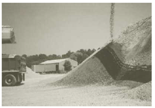
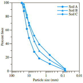
Figure 2.35 (a) Soil-aggregate stockpile; (b) sieve analysis (Courtesy of Khaled Sobhan, Florida Atlantic University, Boca Raton, Florida)
a. Determine the coefficient of uniformity and the coefficient of gradation for Soils A, B, and C.
b. Which one is coarser: Soil A or Soil C? Justify your answer.
c. Although the soils are obtained from the same stockpile, why are the curves so different? (Hint: Comment on particle segregation and representative field sampling.)
d. Determine the percentages of gravel, sand and fines according to Unified Soil Classification System.
(a)
Calculate the coefficient of uniformity
Answer to Problem 2.1CTP
The uniformity coefficient of soil A is
The coefficient of gradation of soil A is
The uniformity coefficient of soil B is
The coefficient of gradation of soil B is
The uniformity coefficient of soil C is
The coefficient of gradation of soil C is
Explanation of Solution
Sketch the grain size distribution curve for soils A, B, and C as shown in Figure 1.
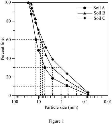
Refer to Figure 1.
For soil A:
The diameter of the particle corresponding to
The diameter of the particle corresponding to
The diameter of the particle corresponding to
For soil B:
The diameter of the particle corresponding to
The diameter of the particle corresponding to
The diameter of the particle corresponding to
For soil C:
The diameter of the particle corresponding to
The diameter of the particle corresponding to
The diameter of the particle corresponding to
Calculate the uniformity coefficient
For soil A:
Substitute
Hence, the uniformity coefficient for soil A is
For soil B:
Substitute
Hence, the uniformity coefficient for soil B is
For soil C:
Substitute
Hence, the uniformity coefficient for soil C is
Calculate the coefficient of gradation
For soil A:
Substitute
Hence, the coefficient of gradation for soil A is
For soil B:
Substitute
Hence, the coefficient of gradation for soil B is
For soil C:
Substitute
Therefore, the coefficient of gradation for soil C is
(b)
State which of the soil is coarser from soil A and C.
Answer to Problem 2.1CTP
Soil A is coarser than soil C.
Explanation of Solution
Refer to part (a).
The uniformity coefficient of soil A is
The uniformity coefficient of soil C is
The percent of soil finer than
The percent of soil finer than
Hence, a higher percentage of soil C is finer than soil A.
Hence, soil A is coarser than soil C.
(c)
Explain the reason for curve different of soil A, B and C if it is obtained from same stockpile.
Explanation of Solution
The particle-size distribution curve shows the range of particle sizes present in a soil and the type of distribution of various-size particles.
Refer to Figure 1.
Particle separation of coarser and finer particles may take place in aggregate stockpiles. This makes representative sampling difficult.
Therefore, the particle-size distribution curve is different for soils A, B, and C.
(d)
Calculate the percentages of gravel, sand, and fines according to the Unified Soil Classification System.
Answer to Problem 2.1CTP
The percentage of gravel for soil A is
The percentage of sand for soil A is
The percentage of fines for soil A is
The percentage of gravel for soil B is
The percentage of sand for soil B is
The percentage of fines for soil B is
The percentage of gravel for soil C is
The percentage of sand for soil C is
The percentage of fines for soil C is
Explanation of Solution
Refer to Figure 1.
For soil A.
The percent passing through
The percent passing through
Calculate the percentage of gravel as shown below.
Hence, the percentage of gravel is
Calculate the percentage of sand as shown below.
Hence, the percentage of sand is
Calculate the percentage of fines as shown below.
Hence, the percentage of fines is
Refer to Figure 1.
For soil B.
The percent passing through
The percent passing through
Calculate the percentage of gravel as shown below.
Hence, the percentage of gravel is
Calculate the percentage of sand as shown below.
Hence, the percentage of sand is
Calculate the percentage of fines as shown below.
Hence, the percentage of fines is
Refer to Figure 1.
For soil C.
The percent passing through
The percent passing through
Calculate the percentage of gravel as shown below.
Hence, the percentage of gravel is
Calculate the percentage of sand as shown below.
Hence, the percentage of sand is
Calculate the percentage of fines as shown below.
Hence, the percentage of fines is
Want to see more full solutions like this?
Chapter 2 Solutions
Principles Of Geotechnical Engineering, Si Edition


- steel designarrow_forwardSITUATION 1: A W250 x 131 is used as a column with an unbraced length of 8 m with respect to the x-x axis and 4 m with respect to the y-y axis. Assume an A36 steel member, pin-connected at the top and fixed at the bottom. Assume that the column is pin connected at mid-height. Use NSCP 2001 NSCP. Fy = 250 MPa. Properties of W250 x 131: A = 16,774 mm² d=274 mm bf=262 mm tf=25 mm tw = 16 mm Ix=222.268 x 10 mm ly = 74.505 x 10° mm* Effective Length Factors: Pinned at both ends, K = 1.0 Pinned at one end and fixed at the other, K = 0.8 1. What is the value of the slenderness ratio to be used for the column? 2. What is the nominal axial stress? 3. What is the design axial load? 1. 60.019 2. 206.543 MPa 3. 3118.091 kNarrow_forwardSITUATION 2: An 8-meter simply supported beam is to be loaded, in addition to its self-weight, a triangular distributed load that linearly increases from zero at the left support to 20 kN/m (dead) + 35 kN/m (live) at the right support. It is braced laterally at the end supports and at midspan. The details for the beam cross-section are given below. Use the LRFD provisions of NSCP 2015. W 540 mm x 150 kg/m: Area, A 19,225 mm² Depth, D = 540 mm Clear Distance between Flanges, h = 455 mm Flange width, bf=310 mm Flange thickness, tf = 20 mm Web thickness, tw 12.5 mm Elastic Section Modulus, Sx = 3.72 x 106 mm³ Plastic Section Modulus, Zx = 4.14 x 10 mm³ Torsional Constant, J = 2.04 x 10% mm* Distance between flange centroids, ho = 520 mm Radius of gyration along y-axis, ry = 72 mm Cb = 1.196 Effective radius of gyration, rts = 85 mm Yield Strength of Steel, Fy = 345 MPa Modulus of Elasticity, E=200 GPa 1. What is the ultimate moment capacity of the beam, in kN-m? 1. 1285.470 kN-marrow_forward
- SITUATION 4: A steel column W 300 x 203 kg/m is subjected to an axial load of 2670 kN. Unbraced length of column is 3m, and assume that the column is pinned at both ends, side sway prevented. Show your complete solution and box only the final answer. Properties of Column: Area, A = 25,740 mm² Depth, d=340 mm Flange thickness, tf = 32 mm Flange Width, bf=315 mm Web thickness, tw = 20 mm Ix = 5.16 x 10 mm² ly = 1.65 x 10° mm* Fy = 345.6 MPa 1. Determine the design strength (kN) of the column. 2. Determine the allowable strength (kN) of the column. 3. What is the value of the slenderness ratio to be used for the column? 1. 7223.401 kN 2. 4805.988 kN 3. 37.470arrow_forwardGive me a steel member design problems under combined axial and bending forces, using interaction equations, with complete solution and final answerarrow_forwardGive me compression member problems in steel design, including calculation of slenderness ratio and critical stress using Euler formula, with complete solution and answer.arrow_forward
- Give me flexural design problems of steel beams, including lateral-torsional buckling, and solve for nominal moment capacity, with step-by-step solution and answer.arrow_forwardGive me a sample tension member problems with staggered bolt holes where I calculate net area using the staggered hole formula, with complete solution and answer.arrow_forwardGive me a block shear failure problem involving a bolted steel plate, and solve for nominal strength, with detailed solution and answer.arrow_forward
- Give me a sample problems computing effective net area of a tension member with staggered holes, with full solution and answer. plsssarrow_forwardCan u pls give me sample problems on steel tension member design involving gross and net area, with complete solution and final answer. Note: I just needed to reviewarrow_forward(a) Determine the Nataf model for the joint PDF fxx, (xx) of the basic (physical) random variables X₁ and X, with marginal PDF's fx(x)=e, 0≤x (Exponential distribution) fx₁ (x2)=x2e-0.5x, 0≤x (Rayleigh distribution) and correlation coefficient Pxx=0.50 Note: Use Table 6 of paper by Liu and Der Kiureghian, 1986. (b) Generate a 3D surface plot and contour plot of the joint PDF fxx, (x,x) using Matlab or any other software of your choice. (c) What is the standard deviation of X2? (d) Construct a transformation from the physical X space (defined by random variables X, and X,) to the standard normal U space (defined by the statistically independent standard normal random variables (U, and U₂), i.e., U=T(X). Also describe the inverse transform X=T(U) and the Jacobian matrices J = ди θα and Ju Ox ди (e) According to the inverse transformation X = T¹ (U) and using Matlab, generate 1,000 samples from the Nataf joint PDF fxx, (x1,x2) derived in part (a). Start by generating samples of U using a…arrow_forward
 Principles of Geotechnical Engineering (MindTap C...Civil EngineeringISBN:9781305970939Author:Braja M. Das, Khaled SobhanPublisher:Cengage Learning
 Traffic and Highway EngineeringCivil EngineeringISBN:9781305156241Author:Garber, Nicholas J.Publisher:Cengage Learning
 Fundamentals of Geotechnical Engineering (MindTap...Civil EngineeringISBN:9781305635180Author:Braja M. Das, Nagaratnam SivakuganPublisher:Cengage Learning
 Construction Materials, Methods and Techniques (M...Civil EngineeringISBN:9781305086272Author:William P. Spence, Eva KultermannPublisher:Cengage Learning
 Principles of Foundation Engineering (MindTap Cou...Civil EngineeringISBN:9781337705028Author:Braja M. Das, Nagaratnam SivakuganPublisher:Cengage Learning