
Videos
For each of the determinants of
The impact of various factors on the demand, supply, and equilibrium price of hybrid gasoline-electric vehicles like Toyota Prius with the help of given supply and demand function.
Explanation of Solution
The demand curve is the graphical representation of quantity demanded by a consumer at a given price level. The changes in quantity demanded on the demand curve can be determined in two ways.
- Movement along the demand curve: this happens when the price of commodity change while keeping another factor constant. A rise in price leads to an upward movement along the demand curve whereas, when the price falls it leads to a downward movement along the demand curve.
- The shift in the demand curve: when factors other than price changes, demand curve shift either right or left
The demand function for Toyota prius can be expressed as:
Here, QD = quantity demanded of Toyota Prius,
P = price of Toyota prius,
PS = price of Nissan leaf, it is substitutes of Toyota prius,
PC = price of gasoline, which is complementary good for Toyota prius,
Y = income of consumers
A = advertising and promotion expenditures by Toyota
AC = competitors’ advertising and promotion expenditures
N = size of the potential target market
CP = consumer tastes and preferences for Toyota,
PE = expected future price appreciation or depreciation Toyota prius,
TA = purchase adjustment time period
T/S = taxes or subsidies on Toyota.
As demand for good increases (decreases), it will lead to increase (decrease) the equilibrium price of that good.
These are the factors that can impact the demand for Toyota prius (TP) in following manner:
| Factors | Result of change in factors | Equilibrium price: increase or decrease. |
| Increase (decrease) in price of Toyota prius | Decrease (increase) in quantity demanded for TP. | - |
| Increase (decrease) in price of Nissan leaf | Increase (decrease) in demand for TP. | Increase (decrease) in equilibrium price of TP. |
| Increase (decrease) in price of gasoline | Decrease (increase) in demand for TP. | Decrease (increase) in equilibrium price of TP. |
| Increase (decrease) in income of consumers | Increase (decrease) in demand for TP. | Increase (decrease) in equilibrium price of TP. |
| Increase (decrease) in advertising and promotion expenditures by Toyota | Increase (decrease) in demand for TP. | Increase (decrease) in equilibrium price of TP. |
| Increase (decrease) in competitors’ advertising and promotion expenditures | Decrease (increase) in demand for TP. | Decrease (increase) in equilibrium price of TP. |
| Increase (decrease) in size of the potential target market | Increase (decrease) in demand for TP. | Increase (decrease) in equilibrium price of TP. |
| Increase (decrease) in consumer tastes and preferences for Toyota | Increase (decrease) in demand for TP. | Increase (decrease) in equilibrium price of TP. |
| Increase (decrease) in expected future price appreciation or depreciation Toyota prius | Increase (decrease) in demand for TP. | Increase (decrease) in equilibrium price of TP. |
| Increase (decrease) in purchase adjustment time period | Increase (decrease) in demand for TP. | Increase (decrease) in equilibrium price of TP. |
| Increase (decrease) in taxes or subsidies on Toyota. | Decrease (increase) in demand for TP. Because of tax, price of TP rises and as a result demand will fall. | Decrease (increase) in equilibrium price of TP. |
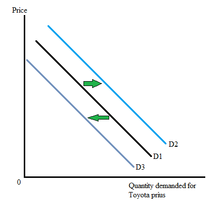
With the help of following graph, the increase and decrease in demand for TP can be seen. As demand for TP increases, the demand curve shifts to the right from D1 to D2. And as demand for TP fall, the demand curve shifts to the left from D1 to D3.
The supply curve is the graphical representation of quantity supplied by a producer at a given price level.
The supply function for Toyota prius (TP) can be expressed as:
Here, Qs = quantity supplied of TP
P = price of the TP
PI = price of inputs like sheet metal
PUI = price of unused substitute inputs like fiberglass
T = technological improvements
EE = entry or exit of other auto sellers
F = accidental supply interruptions from fires, floods, etc.
RC = costs of regulatory compliance
PE = expected (future) changes in price
TA = adjustment time period
T/S = taxes or subsidies
As supply of good increases (decreases), it will lead to decrease (increase) the equilibrium price of that good.
These are the factors that can impact the demand for Toyota prius (TP) in following manner:
| Factors | Result of change in factors | Equilibrium price: increase or decrease. |
| Increase (decrease) in price of Toyota prius | Increase (decrease) in quantity supplied for TP. | Decrease (increase) in equilibrium price of TP. |
| Increase (decrease) in price of inputs like sheet metal | Decrease (increase) in supply of TP. | Increase (decrease) in equilibrium price of TP. |
| Increase (decrease) in price of unused substitute inputs like fiberglass | Decrease (increase) in supply of TP. | Increase (decrease) in equilibrium price of TP. |
| Increase (decrease) in technological improvements | Increase (decrease) in supply of TP. | Decrease (increase) in equilibrium price of TP. |
| Increase (decrease) in entry or exit of other auto sellers | Increase (decrease) in supply of TP. | Decrease (increase) in equilibrium price of TP. |
| Increase (decrease) in accidental supply interruptions from fires, floods, etc. | Decrease (increase) in supply of TP. | Increase (decrease) in equilibrium price of TP. |
| Increase (decrease) in costs of regulatory compliance | Decrease (increase) in supply of TP. | Increase (decrease) in equilibrium price of TP. |
| Increase (decrease) in expected (future) changes in price | Decrease (increase) in supply of TP. | Increase (decrease) in equilibrium price of TP. |
| Increase (decrease) in adjustment time period | Increase (decrease) in supply of TP. | Decrease (increase) in equilibrium price of TP. |
| Increase (decrease) in taxes or subsidies on Toyota. | Decrease (increase) in supply of TP. | Increase (decrease) in equilibrium price of TP. |
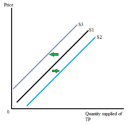
With the help of following graph, the increase and decrease in supply of TP can be seen. As supply of TP increases, the supply curve shifts to the right from S1 to S2. And as supply of TP fall, the supply curve shifts to the left from S1 to S3.
Want to see more full solutions like this?
Chapter 2 Solutions
Bundle: Managerial Economics: Applications, Strategies And Tactics, 14th + Mindtap Economics, 1 Term (6 Months) Printed Access Card


- Recent research indicates potential health benefits associated with coffee consumption, including a potential reduction in the incidence of liver disease. Simultaneously, new technology is being applied to coffee bean harvesting, leading to cost reductions in coffee production. How will these developmentsaffect the demand and supply of coffee? How will the equilibrium price and quantity of coffee change? Use both words and graphs to explain.arrow_forwardRecent research indicates potential health benefits associated with coffee consumption, including a potential reduction in the incidence of liver disease. Simultaneously, new technology is being applied to coffee bean harvesting, leading to cost reductions in coffee production. How will these developmentsaffect the demand and supply of coffee? How will the equilibrium price and quantity of coffee change? Use both words and graphs to explain.arrow_forward► What are the 95% confidence intervals for the intercept and slope in this regression of college grade point average (GPA) on high school GPA? colGPA = 1.39 + .412 hsGPA (.33) (.094)arrow_forward
- G Interpret the following estimated regression equations: wagehr = 0.5+ 2.5exper, where wagehr is the wage, measured in £/hour and exper is years of experience, colGPA = 1.39.412 hsGPA where colGPA is grade point average for a college student, and hsGPA is the grade point average they achieved in high school, cons 124.84 +0.853 inc where cons and inc are annual household consumption and income, both measured in dollars What is (i) the predicted hourly wage for someone with five years of experience? (ii) the predicted grade point average in college for a student whose grade point average in high school was 4.0, (iii) the predicted consumption when household income is $30000? =arrow_forward1. Solving the system of inequalities: I≥3 x+y1 2. Graph y=-2(x+2)(x-3) 3. Please graph the following quadratic inequalities Solve y≤ -1²+2+3arrow_forwardNot use ai pleasearrow_forward
- not use ai pleasearrow_forwardWhat are the key factors that influence the decline of traditional retail businesses in the digital economy? 2. How does consumer behavior impact the success or failure of legacy retail brands? 3. What role does technological innovation play in sustaining long-term competitiveness for retailers? 4. How can traditional retailers effectively adapt their business models to meet evolving market demands?arrow_forwardProblem 1.1 Cyber security is a very costly dimension of doing business for many retailers and their customers who use credit and debit cards. A recent data breach of U.S.-based Home Depot involved some 56 million cardholders. Just to investigate and cover the immediate direct costs of this identity theft amounted to an estimated $62,000,000, of which $27,000,000 was recovered by insurance company payments. This does not include indirect costs, such as, lost future business, costs to banks, and cost to replace cards. If a cyber security vendor had proposed 8 years before the breach that a $10,000,000 investment in a malware detection system could guard the company's computer and payment systems from such a breach, would it have kept up with the rate of inflation estimated at 4% per year?arrow_forward
 Managerial Economics: Applications, Strategies an...EconomicsISBN:9781305506381Author:James R. McGuigan, R. Charles Moyer, Frederick H.deB. HarrisPublisher:Cengage Learning
 Economics (MindTap Course List)EconomicsISBN:9781337617383Author:Roger A. ArnoldPublisher:Cengage Learning


