Videos
a.
Determine the typical seasonal patterns for sales using the ratio-to-moving-average method.
a.
Answer to Problem 28CE
The typical seasonal patterns for sales are 1.191168, 1.121778, 0.435094 and 1.251959, respectively.
Explanation of Solution
Calculation:
Four-Year moving average:
Centered Moving Average:
Specific seasonal index:
| Year | Quarter | Visitors |
Four-quarter moving average |
Centered Moving average | Specific seasonal |
| 2010 | 1 | 210 | |||
| 2 | 180 | ||||
| 3 | 60 | 174.5 | 0.34384 | ||
| 4 | 246 | 174 | 179.5 | 1.370474 | |
| 2011 | 1 | 214 | 175 | 186.75 | 1.145917 |
| 2 | 216 | 184 | 187.5 | 1.152 | |
| 3 | 82 | 189.5 | 189.5 | 0.432718 | |
| 4 | 230 | 185.5 | 195 | 1.179487 | |
| 2012 | 1 | 246 | 193.5 | 197.625 | 1.244782 |
| 2 | 228 | 196.5 | 205 | 1.112195 | |
| 3 | 91 | 198.75 | 212.75 | 0.427732 | |
| 4 | 280 | 211.25 | 217 | 1.290323 | |
| 2013 | 1 | 258 | 214.25 | 222.5 | 1.159551 |
| 2 | 250 | 219.75 | 227.5 | 1.098901 | |
| 3 | 113 | 225.25 | 232.375 | 0.486283 | |
| 4 | 298 | 229.75 | 237.125 | 1.256721 | |
| 2014 | 1 | 279 | 235 | 239.625 | 1.164319 |
| 2 | 267 | 239.25 | 240.75 | 1.109034 | |
| 3 | 116 | 240 | 244.375 | 0.47468 | |
| 4 | 304 | 241.5 | 250.125 | 1.215392 | |
| 2015 | 1 | 302 | 247.25 | 252.75 | 1.194857 |
| 2 | 290 | 253 | 253.25 | 1.145114 | |
| 3 | 114 | 252.5 | 256.375 | 0.444661 | |
| 4 | 310 | 254 | 258.875 | 1.197489 | |
| 2016 | 1 | 321 | 258.75 | 259.75 | 1.235804 |
| 2 | 291 | 259 | 261.75 | 1.111748 | |
| 3 | 120 | 260.5 | |||
| 4 | 320 | 263 |
The Quarterly indexes are,
| I | II | III | IV | |
| 2010 | 0.34384 | 1.370474 | ||
| 2011 | 1.145917 | 1.152 | 0.432718 | 1.179487 |
| 2012 | 1.244782 | 1.112195 | 0.427732 | 1.290323 |
| 2013 | 1.159551 | 1.098901 | 0.486283 | 1.256721 |
| 2014 | 1.164319 | 1.109034 | 0.47468 | 1.215392 |
| 2015 | 1.194857 | 1.145114 | 0.444661 | 1.197489 |
| 2016 | 1.235804 | 1.111748 | ||
| Mean | 1.190871 | 1.121499 | 0.434986 | 1.251648 |
Typical Seasonal index:
Here,
Therefore,
The seasonal indexes are,
| I | II | III | IV | |
| 2010 | 0.34384 | 1.370474 | ||
| 2011 | 1.145917 | 1.152 | 0.432718 | 1.179487 |
| 2012 | 1.244782 | 1.112195 | 0.427732 | 1.290323 |
| 2013 | 1.159551 | 1.098901 | 0.486283 | 1.256721 |
| 2014 | 1.164319 | 1.109034 | 0.47468 | 1.215392 |
| 2015 | 1.194857 | 1.145114 | 0.444661 | 1.197489 |
| 2016 | 1.235804 | 1.111748 | ||
| Mean | 1.190871 | 1.121499 | 0.434986 | 1.251648 |
| Typical Seasonal Index | 1.191168 | 1.121778 | 0.435094 | 1.251959 |
b.
Determine the trend equation.
b.
Answer to Problem 28CE
The trend equation is
Explanation of Solution
Calculation:
Deseasonalization:
| Sales | Typical seasonal index | Deseasonalized Sales |
| 210 | 1.191168 | 176.29755 |
| 180 | 1.121778 | 160.4595562 |
| 60 | 0.435094 | 137.9012351 |
| 246 | 1.251959 | 196.4920576 |
| 214 | 1.191168 | 179.6555985 |
| 216 | 1.121778 | 192.5514674 |
| 82 | 0.435094 | 188.4650214 |
| 230 | 1.251959 | 183.7120864 |
| 246 | 1.191168 | 206.5199871 |
| 228 | 1.121778 | 203.2487711 |
| 91 | 0.435094 | 209.1502066 |
| 280 | 1.251959 | 223.6494965 |
| 258 | 1.191168 | 216.5941328 |
| 250 | 1.121778 | 222.8604947 |
| 113 | 0.435094 | 259.7139928 |
| 298 | 1.251959 | 238.0269641 |
| 279 | 1.191168 | 234.2238878 |
| 267 | 1.121778 | 238.0150083 |
| 116 | 0.435094 | 266.6090546 |
| 304 | 1.251959 | 242.8194534 |
| 302 | 1.191168 | 253.5326671 |
| 290 | 1.121778 | 258.5181738 |
| 114 | 0.435094 | 262.0123468 |
| 310 | 1.251959 | 247.6119426 |
| 321 | 1.191168 | 269.4833978 |
| 291 | 1.121778 | 259.4096158 |
| 120 | 0.435094 | 275.8024703 |
| 320 | 1.251959 | 255.5994246 |
Assign t value as 1 for first quarter of 2010, 2 for the second quarter of 2011 and so on.
Step-by-step procedure to obtain the regression using the Excel:
- Enter the data for Sales and t in Excel sheet.
- Go to Data Menu.
- Click on Data Analysis.
- Select ‘Regression’ and click on ‘OK’
- Select the column of Deseasonalized Sales under ‘Input Y
Range ’. - Select the column of t under ‘Input X Range’.
- Click on ‘OK’.
Output for the Regression obtained using the Excel is as follows:
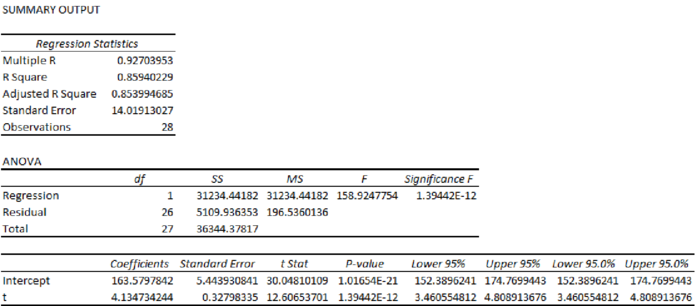
From the Excel output, the regression equation is
c.
Project the sales for the four quarters of next year using the trend equation.
Find the seasonally adjusted values.
c.
Answer to Problem 28CE
The sales for the four quarters for next year are 283.487, 287.6217, 291.7564 and 295.8911.
The seasonally adjusted values are 337.6806, 322.6477, 126.9415 and 370.4435.
Explanation of Solution
Calculation:
From the output, the regression equation is
The t value for first quarter of 2017 is 29.
The t value for second quarter of 2017 is 30.
The t value for third quarter of 2017 is 31.
The t value for fourth quarter of 2017 is 32.
Seasonally Adjusted Forecast:
| Estimated Visitors | Seasonal Index | |
| 283.487 | 1.191168 | 337.6806 |
| 287.6217 | 1.121778 | 322.6477 |
| 291.7564 | 0.435094 | 126.9415 |
| 295.8911 | 1.251959 | 370.4435 |
Want to see more full solutions like this?
Chapter 18 Solutions
EBK STATISTICAL TECHNIQUES IN BUSINESS


- QUAI6221wA1.docx X + int.com/:w:/r/sites/TertiaryStudents/_layouts/15/Doc.aspx?sourcedoc=%7B2759DFAB-EA5E-4526-9991-9087A973B894%7 26 QUAT6221wA1 Q.1.1.8 One advantage of primary data is that: (1) It is low quality (2) It is irrelevant to the purpose at hand (3) It is time-consuming to collect (4) None of the other options Accessibility Mode Immersive R Q.1.1.9 A sample of fifteen apples is selected from an orchard. We would refer to one of these apples as: (2) ھا (1) A parameter (2) A descriptive statistic (3) A statistical model A sampling unit Q.1.1.10 Categorical data, where the categories do not have implied ranking, is referred to as: (2) Search D (2) 1+ PrtSc Insert Delete F8 F10 F11 F12 Backspace 10 ENG USarrow_forwardepoint.com/:w:/r/sites/TertiaryStudents/_layouts/15/Doc.aspx?sourcedoc=%7B2759DFAB-EA5E-4526-9991-9087A 23;24; 25 R QUAT6221WA1 Accessibility Mode DE 2025 Q.1.1.4 Data obtained from outside an organisation is referred to as: (2) 45 (1) Outside data (2) External data (3) Primary data (4) Secondary data Q.1.1.5 Amongst other disadvantages, which type of data may not be problem-specific and/or may be out of date? W (2) E (1) Ordinal scaled data (2) Ratio scaled data (3) Quantitative, continuous data (4) None of the other options Search F8 F10 PrtSc Insert F11 F12 0 + /1 Backspaarrow_forward/r/sites/TertiaryStudents/_layouts/15/Doc.aspx?sourcedoc=%7B2759DFAB-EA5E-4526-9991-9087A973B894%7D&file=Qu Q.1.1.14 QUAT6221wA1 Accessibility Mode Immersive Reader You are the CFO of a company listed on the Johannesburg Stock Exchange. The annual financial statements published by your company would be viewed by yourself as: (1) External data (2) Internal data (3) Nominal data (4) Secondary data Q.1.1.15 Data relevancy refers to the fact that data selected for analysis must be: (2) Q Search (1) Checked for errors and outliers (2) Obtained online (3) Problem specific (4) Obtained using algorithms U E (2) 100% 高 W ENG A US F10 点 F11 社 F12 PrtSc 11 + Insert Delete Backspacearrow_forward
- A client of a commercial rose grower has been keeping records on the shelf-life of a rose. The client sent the following frequency distribution to the grower. Rose Shelf-Life Days of Shelf-Life Frequency fi 1-5 2 6-10 4 11-15 7 16-20 6 21-25 26-30 5 2 Step 2 of 2: Calculate the population standard deviation for the shelf-life. Round your answer to two decimal places, if necessary.arrow_forwardA market research firm used a sample of individuals to rate the purchase potential of a particular product before and after the individuals saw a new television commercial about the product. The purchase potential ratings were based on a 0 to 10 scale, with higher values indicating a higher purchase potential. The null hypothesis stated that the mean rating "after" would be less than or equal to the mean rating "before." Rejection of this hypothesis would show that the commercial improved the mean purchase potential rating. Use = .05 and the following data to test the hypothesis and comment on the value of the commercial. Purchase Rating Purchase Rating Individual After Before Individual After Before 1 6 5 5 3 5 2 6 4 6 9 8 3 7 7 7 7 5 4 4 3 8 6 6 What are the hypotheses?H0: d Ha: d Compute (to 3 decimals).Compute sd (to 1 decimal). What is the p-value?The p-value is What is your decision?arrow_forwardWhy would you use a histograph or bar graph? Which would be better and why for the data shown.arrow_forward
- Please help me with this question on statisticsarrow_forwardPlease help me with this statistics questionarrow_forwardPlease help me with the following statistics questionFor question (e), the options are:Assuming that the null hypothesis is (false/true), the probability of (other populations of 150/other samples of 150/equal to/more data/greater than) will result in (stronger evidence against the null hypothesis than the current data/stronger evidence in support of the null hypothesis than the current data/rejecting the null hypothesis/failing to reject the null hypothesis) is __.arrow_forward
- Please help me with the following question on statisticsFor question (e), the drop down options are: (From this data/The census/From this population of data), one can infer that the mean/average octane rating is (less than/equal to/greater than) __. (use one decimal in your answer).arrow_forwardHelp me on the following question on statisticsarrow_forward3. [15] The joint PDF of RVS X and Y is given by fx.x(x,y) = { x) = { c(x + { c(x+y³), 0, 0≤x≤ 1,0≤ y ≤1 otherwise where c is a constant. (a) Find the value of c. (b) Find P(0 ≤ X ≤,arrow_forwardarrow_back_iosSEE MORE QUESTIONSarrow_forward_ios
 Glencoe Algebra 1, Student Edition, 9780079039897...AlgebraISBN:9780079039897Author:CarterPublisher:McGraw Hill
 Holt Mcdougal Larson Pre-algebra: Student Edition...AlgebraISBN:9780547587776Author:HOLT MCDOUGALPublisher:HOLT MCDOUGAL
 Trigonometry (MindTap Course List)TrigonometryISBN:9781305652224Author:Charles P. McKeague, Mark D. TurnerPublisher:Cengage Learning
 College Algebra (MindTap Course List)AlgebraISBN:9781305652231Author:R. David Gustafson, Jeff HughesPublisher:Cengage Learning
 Big Ideas Math A Bridge To Success Algebra 1: Stu...AlgebraISBN:9781680331141Author:HOUGHTON MIFFLIN HARCOURTPublisher:Houghton Mifflin Harcourt