Videos
a.
Determine the typical seasonal patterns for the production data using the ratio-to-moving-average method.
a.
Answer to Problem 26CE
The typical seasonal patterns for sales are 0.7549, 0.9913, 1.4043 and 0.8495, respectively.
Explanation of Solution
Calculation:
Four-Year moving average:
Centered Moving Average:
Specific seasonal index:
| Year | Quarter | Board ft Millions |
Four-quarter moving average |
Centered Moving average | Specific seasonal |
| 2012 | Winter | 7.8 | |||
| Spring | 10.2 | ||||
| Summer | 14.7 | 10.3875 | 1.41516 | ||
| Fall | 9.3 | 10.5 | 10.45 | 0.88995 | |
| 2013 | Winter | 6.9 | 10.275 | 10.975 | 0.6287 |
| Spring | 11.6 | 10.625 | 11.325 | 1.02428 | |
| Summer | 17.5 | 11.325 | 11.575 | 1.51188 | |
| Fall | 9.3 | 11.325 | 11.5875 | 0.80259 | |
| 2014 | Winter | 8.9 | 11.825 | 11.075 | 0.80361 |
| Spring | 9.7 | 11.35 | 10.9 | 0.88991 | |
| Summer | 15.3 | 10.8 | 11.225 | 1.36303 | |
| Fall | 10.1 | 11 | 11.7875 | 0.85684 | |
| 2015 | Winter | 10.7 | 11.45 | 12.3125 | 0.86904 |
| Spring | 12.4 | 12.125 | 12.575 | 0.98608 | |
| Summer | 16.8 | 12.5 | 12.4625 | 1.34804 | |
| Fall | 10.7 | 12.65 | 12.425 | 0.86117 | |
| 2016 | Winter | 9.2 | 12.275 | 12.6125 | 0.72944 |
| Spring | 13.6 | 12.575 | 12.6 | 1.07937 | |
| Summer | 17.1 | 12.65 | |||
| Fall | 10.3 | 12.55 |
The Quarterly indexes are,
| Winter | Spring | Summer | Fall | |
| 2012 | 1.415162 | 0.889952 | ||
| 2013 | 0.628702 | 1.024283 | 1.511879 | 0.802589 |
| 2014 | 0.803612 | 0.889908 | 1.363029 | 0.85684 |
| 2015 | 0.869036 | 0.986083 | 1.348044 | 0.861167 |
| 2016 | 0.729435 | 1.079365 | ||
| Mean | 0.757696 | 0.99491 | 1.409529 | 0.852637 |
Typical Seasonal index:
Here,
Therefore,
The typical seasonal indexes are,
| Winter | Spring | Summer | Fall | |
| 2012 | 1.415162 | 0.889952 | ||
| 2013 | 0.628702 | 1.024283 | 1.511879 | 0.802589 |
| 2014 | 0.803612 | 0.889908 | 1.363029 | 0.85684 |
| 2015 | 0.869036 | 0.986083 | 1.348044 | 0.861167 |
| 2016 | 0.729435 | 1.079365 | ||
| Mean | 0.757696 | 0.99491 | 1.409529 | 0.852637 |
| Typical Index | 0.7549 | 0.9913 | 1.4043 | 0.8495 |
b.
Interpret the typical seasonal pattern.
b.
Explanation of Solution
The typical seasonal index for the Summer quarter is 1.4043, which is largest compared with other three quarters. That is, the production is largest in the third quarter and moreover, it represent above the average quarters because seasonal index is greater than 1. The Winter, Spring and Fall quarters represent below the average quarters because seasonal indexes for the three quarters are less than 1.
c.
Determine the trend equation.
c.
Answer to Problem 26CE
The trend equation is
Explanation of Solution
Calculation:
Deseasonalization:
| Board ft Millions | Typical Seasonal Index | Deseasonalized production |
| 7.8 | 0.7549 | 10.33249437 |
| 10.2 | 0.9913 | 10.28951881 |
| 14.7 | 1.4043 | 10.46784875 |
| 9.3 | 0.8495 | 10.94761624 |
| 6.9 | 0.7549 | 9.140283481 |
| 11.6 | 0.9913 | 11.70180571 |
| 17.5 | 1.4043 | 12.4617247 |
| 9.3 | 0.8495 | 10.94761624 |
| 8.9 | 0.7549 | 11.78964101 |
| 9.7 | 0.9913 | 9.785130637 |
| 15.3 | 1.4043 | 10.89510788 |
| 10.1 | 0.8495 | 11.88934667 |
| 10.7 | 0.7549 | 14.17406279 |
| 12.4 | 0.9913 | 12.50882679 |
| 16.8 | 1.4043 | 11.96325571 |
| 10.7 | 0.8495 | 12.5956445 |
| 9.2 | 0.7549 | 12.18704464 |
| 13.6 | 0.9913 | 13.71935842 |
| 17.1 | 1.4043 | 12.17688528 |
| 10.3 | 0.8495 | 12.12477928 |
Assign t value as 1 for first quarter of 2012, 2 for the second quarter of 2012 and so on.
Step-by-step procedure to obtain the regression using the Excel:
- Enter the data for Deseasonalized production and t in Excel sheet.
- Go to Data Menu.
- Click on Data Analysis.
- Select ‘Regression’ and click on ‘OK’
- Select the column of Deseasonalized production under ‘Input Y
Range ’. - Select the column of t under ‘Input X Range’.
- Click on ‘OK’.
Output for the Regression obtained using the Excel is as follows:
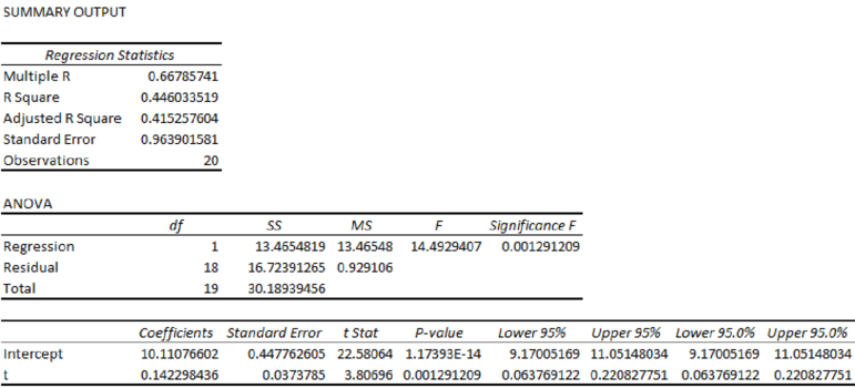
From the Excel output, the regression equation is
d.
Find the seasonally adjusted production for four quarters of 2017.
d.
Answer to Problem 26CE
The seasonally adjusted production for four quarters of 2017 are 9.8884, 13.1261, 18.7946 and 11.4903, respectively.
Explanation of Solution
Calculation:
From the output, the regression equation is
The t value for first quarter of 2017 is 21.
The t value for second quarter of 2017 is 22.
The t value for third quarter of 2017 is 23.
The t value for fourth quarter of 2017 is 24.
Seasonally Adjusted Forecast:
| Estimated Visitors | Seasonal Index | |
| 13.0990 | 0.7549 | 9.8884 |
| 13.2413 | 0.9913 | 13.1261 |
| 13.3836 | 1.4043 | 18.7946 |
| 13.5259 | 0.8495 | 11.4903 |
Want to see more full solutions like this?
Chapter 18 Solutions
EBK STATISTICAL TECHNIQUES IN BUSINESS


- Let Y₁, Y2,, Yy be random variables from an Exponential distribution with unknown mean 0. Let Ô be the maximum likelihood estimates for 0. The probability density function of y; is given by P(Yi; 0) = 0, yi≥ 0. The maximum likelihood estimate is given as follows: Select one: = n Σ19 1 Σ19 n-1 Σ19: n² Σ1arrow_forwardPlease could you help me answer parts d and e. Thanksarrow_forwardWhen fitting the model E[Y] = Bo+B1x1,i + B2x2; to a set of n = 25 observations, the following results were obtained using the general linear model notation: and 25 219 10232 551 XTX = 219 10232 3055 133899 133899 6725688, XTY 7361 337051 (XX)-- 0.1132 -0.0044 -0.00008 -0.0044 0.0027 -0.00004 -0.00008 -0.00004 0.00000129, Construct a multiple linear regression model Yin terms of the explanatory variables 1,i, x2,i- a) What is the value of the least squares estimate of the regression coefficient for 1,+? Give your answer correct to 3 decimal places. B1 b) Given that SSR = 5550, and SST=5784. Calculate the value of the MSg correct to 2 decimal places. c) What is the F statistics for this model correct to 2 decimal places?arrow_forward
- Calculate the sample mean and sample variance for the following frequency distribution of heart rates for a sample of American adults. If necessary, round to one more decimal place than the largest number of decimal places given in the data. Heart Rates in Beats per Minute Class Frequency 51-58 5 59-66 8 67-74 9 75-82 7 83-90 8arrow_forwardcan someone solvearrow_forwardQUAT6221wA1 Accessibility Mode Immersiv Q.1.2 Match the definition in column X with the correct term in column Y. Two marks will be awarded for each correct answer. (20) COLUMN X Q.1.2.1 COLUMN Y Condenses sample data into a few summary A. Statistics measures Q.1.2.2 The collection of all possible observations that exist for the random variable under study. B. Descriptive statistics Q.1.2.3 Describes a characteristic of a sample. C. Ordinal-scaled data Q.1.2.4 The actual values or outcomes are recorded on a random variable. D. Inferential statistics 0.1.2.5 Categorical data, where the categories have an implied ranking. E. Data Q.1.2.6 A set of mathematically based tools & techniques that transform raw data into F. Statistical modelling information to support effective decision- making. 45 Q Search 28 # 00 8 LO 1 f F10 Prise 11+arrow_forward
- Students - Term 1 - Def X W QUAT6221wA1.docx X C Chat - Learn with Chegg | Cheg X | + w:/r/sites/TertiaryStudents/_layouts/15/Doc.aspx?sourcedoc=%7B2759DFAB-EA5E-4526-9991-9087A973B894% QUAT6221wA1 Accessibility Mode பg Immer The following table indicates the unit prices (in Rands) and quantities of three consumer products to be held in a supermarket warehouse in Lenasia over the time period from April to July 2025. APRIL 2025 JULY 2025 PRODUCT Unit Price (po) Quantity (q0)) Unit Price (p₁) Quantity (q1) Mineral Water R23.70 403 R25.70 423 H&S Shampoo R77.00 922 R79.40 899 Toilet Paper R106.50 725 R104.70 730 The Independent Institute of Education (Pty) Ltd 2025 Q Search L W f Page 7 of 9arrow_forwardCOM WIth Chegg Cheg x + w:/r/sites/TertiaryStudents/_layouts/15/Doc.aspx?sourcedoc=%7B2759DFAB-EA5E-4526-9991-9087A973B894%. QUAT6221wA1 Accessibility Mode Immersi The following table indicates the unit prices (in Rands) and quantities of three meals sold every year by a small restaurant over the years 2023 and 2025. 2023 2025 MEAL Unit Price (po) Quantity (q0)) Unit Price (P₁) Quantity (q₁) Lasagne R125 1055 R145 1125 Pizza R110 2115 R130 2195 Pasta R95 1950 R120 2250 Q.2.1 Using 2023 as the base year, compute the individual price relatives in 2025 for (10) lasagne and pasta. Interpret each of your answers. 0.2.2 Using 2023 as the base year, compute the Laspeyres price index for all of the meals (8) for 2025. Interpret your answer. Q.2.3 Using 2023 as the base year, compute the Paasche price index for all of the meals (7) for 2025. Interpret your answer. Q Search L O W Larrow_forwardQUAI6221wA1.docx X + int.com/:w:/r/sites/TertiaryStudents/_layouts/15/Doc.aspx?sourcedoc=%7B2759DFAB-EA5E-4526-9991-9087A973B894%7 26 QUAT6221wA1 Q.1.1.8 One advantage of primary data is that: (1) It is low quality (2) It is irrelevant to the purpose at hand (3) It is time-consuming to collect (4) None of the other options Accessibility Mode Immersive R Q.1.1.9 A sample of fifteen apples is selected from an orchard. We would refer to one of these apples as: (2) ھا (1) A parameter (2) A descriptive statistic (3) A statistical model A sampling unit Q.1.1.10 Categorical data, where the categories do not have implied ranking, is referred to as: (2) Search D (2) 1+ PrtSc Insert Delete F8 F10 F11 F12 Backspace 10 ENG USarrow_forward
- epoint.com/:w:/r/sites/TertiaryStudents/_layouts/15/Doc.aspx?sourcedoc=%7B2759DFAB-EA5E-4526-9991-9087A 23;24; 25 R QUAT6221WA1 Accessibility Mode DE 2025 Q.1.1.4 Data obtained from outside an organisation is referred to as: (2) 45 (1) Outside data (2) External data (3) Primary data (4) Secondary data Q.1.1.5 Amongst other disadvantages, which type of data may not be problem-specific and/or may be out of date? W (2) E (1) Ordinal scaled data (2) Ratio scaled data (3) Quantitative, continuous data (4) None of the other options Search F8 F10 PrtSc Insert F11 F12 0 + /1 Backspaarrow_forward/r/sites/TertiaryStudents/_layouts/15/Doc.aspx?sourcedoc=%7B2759DFAB-EA5E-4526-9991-9087A973B894%7D&file=Qu Q.1.1.14 QUAT6221wA1 Accessibility Mode Immersive Reader You are the CFO of a company listed on the Johannesburg Stock Exchange. The annual financial statements published by your company would be viewed by yourself as: (1) External data (2) Internal data (3) Nominal data (4) Secondary data Q.1.1.15 Data relevancy refers to the fact that data selected for analysis must be: (2) Q Search (1) Checked for errors and outliers (2) Obtained online (3) Problem specific (4) Obtained using algorithms U E (2) 100% 高 W ENG A US F10 点 F11 社 F12 PrtSc 11 + Insert Delete Backspacearrow_forwardA client of a commercial rose grower has been keeping records on the shelf-life of a rose. The client sent the following frequency distribution to the grower. Rose Shelf-Life Days of Shelf-Life Frequency fi 1-5 2 6-10 4 11-15 7 16-20 6 21-25 26-30 5 2 Step 2 of 2: Calculate the population standard deviation for the shelf-life. Round your answer to two decimal places, if necessary.arrow_forward
 Glencoe Algebra 1, Student Edition, 9780079039897...AlgebraISBN:9780079039897Author:CarterPublisher:McGraw Hill
 Holt Mcdougal Larson Pre-algebra: Student Edition...AlgebraISBN:9780547587776Author:HOLT MCDOUGALPublisher:HOLT MCDOUGAL
 Trigonometry (MindTap Course List)TrigonometryISBN:9781305652224Author:Charles P. McKeague, Mark D. TurnerPublisher:Cengage Learning
 College Algebra (MindTap Course List)AlgebraISBN:9781305652231Author:R. David Gustafson, Jeff HughesPublisher:Cengage Learning
 Functions and Change: A Modeling Approach to Coll...AlgebraISBN:9781337111348Author:Bruce Crauder, Benny Evans, Alan NoellPublisher:Cengage Learning