![Loose-Leaf for Financial and Managerial Accounting](https://www.bartleby.com/isbn_cover_images/9781260004861/9781260004861_largeCoverImage.gif)
Loose-Leaf for Financial and Managerial Accounting
7th Edition
ISBN: 9781260004861
Author: John J Wild, Ken W. Shaw, Barbara Chiappetta Fundamental Accounting Principles
Publisher: McGraw-Hill Education
expand_more
expand_more
format_list_bulleted
Textbook Question
Chapter 18, Problem 1E
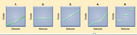
Following are five graphs representing various cost behaviors. (1) Identify whether the cost behavior in each graph is mixed, step-wise, fixed, variable, or curvilinear. (2) Identify the graph (by number) that includes the standard monthly charge plus a charge for each kilowatt hour; (d)
commissions to salespersons; and (e) costs of hourly paid workers that provide substantial gains in efficiency when a few workers are added but gradually smaller gains in efficiency when more workers are added.
______________________________________________________________________________
Expert Solution & Answer
![Check Mark](/static/check-mark.png)
Want to see the full answer?
Check out a sample textbook solution![Blurred answer](/static/blurred-answer.jpg)
Students have asked these similar questions
Matching graphs with descriptions of cost and revenue behavior. (D. Green, adapted) Given here are a number of graphs. The horizontal axis of each graph represents the units produced over the year, and the vertical axis represents total cost or revenues.
Indicate by number which graph best fits the situation or item described (a–h). Some graphs may be used more than once; some may not apply to any of the situations.
Direct material costs
Supervisors’ salaries for one shift and two shifts
A cost-volume-profit graph
Mixed costs—for example, car rental fixed charge plus a rate per mile driven
Depreciation of plant, computed on a straight-line basis
Data supporting the use of a variable-cost rate, such as manufacturing labor cost of $14 per unit produced
Incentive bonus plan that pays managers $0.10 for every unit produced above some level of production
Interest expense on $2 million borrowed at a fixed rate of interest
Based on the image below for a manufacturing company, the correct statement is
A. line b graphs total fixed costs
B. point c represents the point at which the marginal contribution per unit increases
C. line d graphs total costs
D. area e (between lines b and d) represents the contribution margin
The following diagram is a cost-volume-profit graph for a manufacturing company:
^
O
Volume
с
Select the answer that best describes the labeled item on the diagram.
A. Area CDE represents the area of net loss.
B. Line AC graphs total fixed costs.
C. Point D represents a point at which the profit is greater than zero.
D. Line AC graphs total costs.
Chapter 18 Solutions
Loose-Leaf for Financial and Managerial Accounting
Ch. 18 - Prob. 1MCQCh. 18 - Prob. 2MCQCh. 18 - Prob. 3MCQCh. 18 - Prob. 4MCQCh. 18 - Prob. 5MCQCh. 18 - Prob. 1DQCh. 18 - Prob. 2DQCh. 18 - When output volume increases, do fixed costs per...Ch. 18 - How is the cost-volume-profit analysis useful?Ch. 18 - Prob. 5DQ
Ch. 18 - Prob. 6DQCh. 18 - Prob. 7DQCh. 18 - Prob. 8DQCh. 18 - Prob. 9DQCh. 18 - Prob. 10DQCh. 18 - Prob. 11DQCh. 18 - Prob. 12DQCh. 18 - Prob. 13DQCh. 18 - Prob. 14DQCh. 18 - Prob. 15DQCh. 18 - Prob. 16DQCh. 18 - Prob. 17DQCh. 18 - Prob. 18DQCh. 18 - Prob. 19DQCh. 18 - APPLE Should Apple use single product or...Ch. 18 - Prob. 21DQCh. 18 - Prob. 22DQCh. 18 - Prob. 1QSCh. 18 - Prob. 2QSCh. 18 - Cost behavior estimation---high-low method P1 The...Ch. 18 - Prob. 4QSCh. 18 - Prob. 5QSCh. 18 - Prob. 6QSCh. 18 - Prob. 7QSCh. 18 - Prob. 8QSCh. 18 - Prob. 9QSCh. 18 - Prob. 10QSCh. 18 - Prob. 11QSCh. 18 - Prob. 12QSCh. 18 - Prob. 13QSCh. 18 - Prob. 14QSCh. 18 - Prob. 15QSCh. 18 - Prob. 16QSCh. 18 - Prob. 17QSCh. 18 - Prob. 18QSCh. 18 - Prob. 19QSCh. 18 - Prob. 20QSCh. 18 - Prob. 21QSCh. 18 - Following are five graphs representing various...Ch. 18 - Prob. 2ECh. 18 - Prob. 3ECh. 18 - Prob. 4ECh. 18 - Prob. 5ECh. 18 - Prob. 6ECh. 18 - Prob. 7ECh. 18 - Prob. 8ECh. 18 - Prob. 9ECh. 18 - Prob. 10ECh. 18 - Prob. 11ECh. 18 - Prob. 12ECh. 18 - Prob. 13ECh. 18 - Prob. 14ECh. 18 - Prob. 15ECh. 18 - Prob. 16ECh. 18 - Prob. 17ECh. 18 - Prob. 18ECh. 18 - Prob. 19ECh. 18 - Prob. 20ECh. 18 - Prob. 21ECh. 18 - Prob. 22ECh. 18 - Prob. 23ECh. 18 - Prob. 24ECh. 18 - Prob. 25ECh. 18 - Prob. 26ECh. 18 - Prob. 27ECh. 18 - Prob. 1PSACh. 18 - Prob. 2PSACh. 18 - Prob. 3PSACh. 18 - Prob. 4PSACh. 18 - Prob. 5PSACh. 18 - Prob. 6PSACh. 18 - Prob. 7PSACh. 18 - Prob. 1PSBCh. 18 - Prob. 2PSBCh. 18 - Prob. 3PSBCh. 18 - Prob. 4PSBCh. 18 - Prob. 5PSBCh. 18 - Prob. 6PSBCh. 18 - Prob. 7PSBCh. 18 - Prob. 18SPCh. 18 - Apple offers extended service contracts that...Ch. 18 - Prob. 2BTNCh. 18 - Prob. 3BTNCh. 18 - Prob. 4BTNCh. 18 - Prob. 5BTNCh. 18 - Prob. 6BTNCh. 18 - Prob. 7BTNCh. 18 - Prob. 8BTNCh. 18 - Prob. 9BTN
Knowledge Booster
Learn more about
Need a deep-dive on the concept behind this application? Look no further. Learn more about this topic, accounting and related others by exploring similar questions and additional content below.Similar questions
- A CVP graph such as the one shown below is a useful technique for showing relationships among an organization's costs, volume, and profits. 8. Required: Identify the numbered components in the CVP graph. Answer Number 1 Number 2 Number 3 Number 4 Number 5 Number 6 Number 7 Number 8 Number 9 State the effect of each of the following actions on the break-even point. Answer |The unit selling price is increased from $ 18 to $20. |Unit variable expenses are decreased from $12 to $10. |Fixed expenses are increased by $3,000 per period Two thousand more units are sold during the period than were budgeted Due to paying salespersons a commission rather than a flat salary, fixed expenses are reduced by $8,000 per period and unit variable expenses are increased by $3 Due to an increase in the cost of materials, both unit variable expenses and the selling price are increased by $2. Advertising costs are increased by $10,000 per period, resulting in a 10% increase in the number of units sold. Due…arrow_forwardUsing the data in P4-2 and Microsoft Excel: 1. Separate the variable and fixed elements. 2. Determine the cost to be charged to the product for the year. 3. Determine the cost to be charged to factory overhead for the year. 4. Determine the plotted data points using Chart Wizard. 5. Determine R2. 6. How do these solutions compare to the solutions in P4-2 and P4-3? 7. What does R2 tell you about this cost model?arrow_forwardThe Cobb-Douglas production function is a classic model from economics used to model output as a function of capital and labor. It has the form: f(L,C)=c0Lc1Cc2, where c0, c1, and c2 are constants. The variable L represents the units of input of labor, and the variable C represents the units of input of capital. a. In this example, assume c0 = 5, c1 = 0.25, and c2 = 0.75. Assume each unit of labor costs 25 and each unit of capital costs 75. With 75,000 available in the budget, develop an optimization model to determine how the budgeted amount should be allocated between capital and labor in order to maximize output. b. Find the optimal solution to the model you formulated in part (a). (Hint: When using Excel Solver, use the Multistart option with bounds 0 L 3,000 and 0 C 1,000.)arrow_forward
- Explain the concept of customer profitability analysis. Give examples of cost drivers used in this analysis. (500 words)arrow_forwardplease solve with full workarrow_forwardWe have seen how cost and volume assumptions affect net income. A common application of CVP analysis is a tool to forecast sales, costs, and income. Assume that you are actively searching for a job. Identify and discuss three assumptions relating to your expected revenue (salary), and three assumptions related to your expected costs (expenses) for the first year on the job.arrow_forward
- a. Compute labor productivity under each system. Use carts per worker per hour as the measure of labor productivity. (Round your answers to 3 decimal places.) Before After carts per worker per hour carts per worker per hour b. Compute the multifactor productivity under each system. Use carts per dollar cost (labor plus equipment) as the measure. (Round your answers to 3 decimal places.) Before After carts/dollar cost carts/dollar cost c. Comment on the changes in productivity according to the two measures. Round your intermediate calculations to 3 decimal places and final answers to 2 decimal places. Labor productivity Multifactor productivity (Click to select) by (Click to select) byarrow_forwardANSWER ALL THE GIVEN ITEMS. Write “True” if the statement is true and write “False” if the statement is false. 2. A variable cost will change in total in proportion to changes in the level of activity.3. A fixed cost is constant per unit of product.4. Cost accumulation, cost allocation, and cost objects are interrelated.5. A variable cost remains constant per unit, though in total increases as activity levels increase.6. If volume increases, both total variables and total fixed costs will increase.7. Decrease in the level of activity will cause total variable and total fixed costs to decrease.8. When graphed, total variable costs and total fixed costs are both assumed to be linear withinthe relevant range.9. Fixed cost is constant in total amount regardless of changes in activity level within the relevantrange.10. Cost function is an express that mathematically links costs, their behavior, and their cost driver.11. As volume decreases within the relevant range, variable cost per unit…arrow_forwardA supply chain has the following information:(a). Compute the total supply chain throughput time for all the entities from beginning to end.b. Compute the cash-to-cash cycle time for each of thefour entities separately. Based on this calculation, who is benefiting the most?c. Compute the total delivered unit cost in the supplychain from beginning to end. How much profit isthere in the supply chain?arrow_forward
- Data table Month Total Cost Machine Hours January.. 3,420 1,090 February..... S 3,760 1,120 March .... $ 3,532 1,080 April ..... 3,720 1,220 May S 4,800 1,330 June 4,192 1,480 .. %24 %24arrow_forwardVarious cost-behavior patterns. (CPA, adapted). The vertical axes of the graphs below represent total cost, and the horizontal axes represent units produced during a calendar year. In each case, the zero point of dollars and production is at the intersection of the two axes. Select the graph that matches the numbered manufacturing cost data (requirements 1-9). Indicate by letter which graph best fits the situation or item described. The graphs may be used more than once. Annual depreciation of equipment, where the amount of depreciation charged is computed by the machine-hours method. Electricity bill—a flat fixed charge, plus a variable cost after a certain number of kilowatt-hours are used, in which the quantity of kilowatt-hours used varies proportionately with quantity of units produced. City water bill, which is computed as follows: First 1,000,000 gallons or less $1,000 flat fee Next 10,000 gallons $0.003 per gallon used Next 10,000 gallons $0.006 per gallon used Next 10,000…arrow_forwardFill in the missing amounts in each of the eight case situations below. Each case is independent of the others. (Hint: One way to find the missing amounts would be to prepare a contribution format income statement for each case, enter the known data, and then compute the missing items.) Required: a. Assume that only one product is being sold in each of the following four case situations: Unit sold Sales Variable expenses Foxed expenses Operating income (loss) Contribution margin per unit $ Case #1 15,000 180,000 $ 100,000 120,000 50,000 $ $ Case #2 Case #1 Case #3 10,000 Case #2 70,000 $ 32,000 8,000 $ 12,000 $ 10 $ 13 Case #4 b. Assume that more than one product is being sold in each of the following four case situations: (Enter "Contribution margin ratio" in percent. Round your final answers to the nearest whole dollar amount.) Case #3 6,000 300,000 100,000 (10,000) Case #4arrow_forward
arrow_back_ios
SEE MORE QUESTIONS
arrow_forward_ios
Recommended textbooks for you
- Principles of Cost AccountingAccountingISBN:9781305087408Author:Edward J. Vanderbeck, Maria R. MitchellPublisher:Cengage LearningEssentials of Business Analytics (MindTap Course ...StatisticsISBN:9781305627734Author:Jeffrey D. Camm, James J. Cochran, Michael J. Fry, Jeffrey W. Ohlmann, David R. AndersonPublisher:Cengage LearningPrinciples of Accounting Volume 2AccountingISBN:9781947172609Author:OpenStaxPublisher:OpenStax College
- Excel Applications for Accounting PrinciplesAccountingISBN:9781111581565Author:Gaylord N. SmithPublisher:Cengage Learning
![Text book image](https://www.bartleby.com/isbn_cover_images/9781305087408/9781305087408_smallCoverImage.gif)
Principles of Cost Accounting
Accounting
ISBN:9781305087408
Author:Edward J. Vanderbeck, Maria R. Mitchell
Publisher:Cengage Learning
![Text book image](https://www.bartleby.com/isbn_cover_images/9781305627734/9781305627734_smallCoverImage.gif)
Essentials of Business Analytics (MindTap Course ...
Statistics
ISBN:9781305627734
Author:Jeffrey D. Camm, James J. Cochran, Michael J. Fry, Jeffrey W. Ohlmann, David R. Anderson
Publisher:Cengage Learning
Principles of Accounting Volume 2
Accounting
ISBN:9781947172609
Author:OpenStax
Publisher:OpenStax College
![Text book image](https://www.bartleby.com/isbn_cover_images/9781111581565/9781111581565_smallCoverImage.gif)
Excel Applications for Accounting Principles
Accounting
ISBN:9781111581565
Author:Gaylord N. Smith
Publisher:Cengage Learning
alue Chain Analysis EXPLAINED | B2U | Business To You; Author: Business To You;https://www.youtube.com/watch?v=SI5lYaZaUlg;License: Standard Youtube License