Chapter 17, Problem 18P

 (a)

To determine

The total marginal benefit $\left({\text{MB}}_{\text{T}}\right)$.

Explanation of Solution

The total marginal benefit (MB) is the sum total of individual marginal benefits. There are two consumers of mosquito abatement, such as D and L, where the marginal benefit of consumer D is ${\text{MB}}_{\text{D}}=100-\text{Q}$ and the marginal benefit of consumer L is ${\text{MB}}_{\text{L}}=60-\text{Q}$. Therefore, the total marginal benefit can be calculated as follows:

$\begin{array}{c}{\text{MB}}_{\text{T}}={\text{MB}}_{\text{D}}+{\text{MB}}_{\text{L}}\\ =100-\text{Q}+60-\text{Q}\\ =160-2\text{Q}\end{array}$

Therefore, the total marginal benefit is ${\text{MB}}_{\text{T}}=160-2\text{Q}$.

Economics Concept Introduction

Marginal benefit: Marginal benefit can be defined as the additional utility derived from the additional consumption of one or more unit of goods and services.

 (b)

To determine

The optimal level of mosquito abatement.

Explanation of Solution

The optimal level of mosquito abatement is determined at the point where the total marginal benefit is equal to the marginal cost (MC).

The total marginal benefit is ${\text{MB}}_{\text{T}}=160-2\text{Q}$.

The total marginal cost is given as $\text{MC}=2\text{Q}$.

Now, set the two expressions to get the value of optimal quantity:

$\begin{array}{c}160-2\text{Q}=2\text{Q}\\ 160=4\text{Q}\\ \text{Q}=\frac{160}{4}\\ =40\end{array}$

Therefore, the optimal level of mosquito abatement is 40.

Economics Concept Introduction

Marginal benefit: Marginal benefit can be defined as the additional utility derived from the additional consumption of one or more unit of goods and services.

Marginal cost (MC): Marginal benefit refers to the amount of additional cost incurred in the process of increasing one more unit of output.

 (c)

To determine

The individual total benefit at the optimal level of mosquito abatement.

Explanation of Solution

Figure 1 illustrates the MB, MC, and the optimal quantity of the mosquito abatement of consumer D as follows:

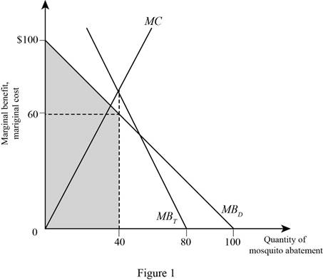
In Figure1, the vertical axis shows the MB and MC of the mosquito abatement and the horizontal axis shows the quantity of mosquito abatement, where the interaction between the total marginal benefit with MC curve determines the optimal quantity of mosquito abatement.

The MB of consumer D can be calculated by substituting the respective value in the MB function of D as follows:

  $\begin{array}{c}{\text{MB}}_{\text{D}}=\left(100-40\right)\\ =60\end{array}$

Therefore, 60 is the MB of consumer D.

The MB of consumer L can be calculated by substituting the respective value in the MB function of L as follows:

$\begin{array}{c}{\text{MB}}_{\text{L}}=\left(60-40\right)\\ =20\end{array}$

Therefore, 20 is the MB of consumer D.

Therefore, the total benefit is 80$\left(60+20\right)$.

Now, the total benefit (TB) for consumer D can be calculated using the formula given below:

$\begin{array}{c}\text{TB}=\text{Optimal quantity}\times {\text{MB}}_{\text{D}}+\frac{1}{2}\times \text{Optimal }\\ \text{quantity}\times \left({\text{MB}}_{\text{D}}-{\text{MB}}_{\text{L}}\right)\end{array}$ (1)

Now, substitute the respective values in Equation (1) to get the value of total benefit of consumer D.

$\begin{array}{c}\text{TB}=40\times 60+\frac{1}{2}\times 40\times \left(60-20\right)\\ =3,200\end{array}$

Therefore, the total benefit of consumer D is 3,200.

Figure 2 illustrates the MB, MC, and the optimal quantity of the mosquito abatement of consumer L as follows:

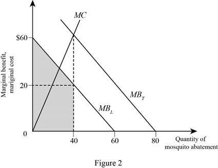
In Figure2, the vertical axis measures the MB and MC of the mosquito abatement and the horizontal axis measures the quantity of mosquito abatement, where the interaction between the total marginal benefit with MC curve determines the optimal quantity of mosquito abatement.

The total benefit (TB) for consumer L can be calculated using the formula given below:

$\begin{array}{c}\text{TB}=\text{Optimal quantity}\times {\text{MB}}_{\text{L}}+\frac{1}{2}\times \text{Optimal }\\ \text{quantity}\times \left({\text{MB}}_{\text{D}}-{\text{MB}}_{\text{L}}\right)\end{array}$ (2)

Now, substitute the respective values in Equation (2) to get the value of total benefit of consumer L.

$\begin{array}{c}\text{TB}=40\times 20+\frac{1}{2}\times 40\times \left(60-20\right)\\ =1,600\end{array}$

Therefore, the total benefit of consumer L is 1,600.

Economics Concept Introduction

Marginal benefit: Marginal benefit can be defined as the additional utility derived from the additional consumption of one or more unit of goods and services.

Marginal cost (MC): Marginal benefit refers to the amount of additional cost incurred in the process of increasing one more unit of output.