Videos
Refer to the Baseball 2012 data, which report information on the 2012 Major League Baseball season.
- a. Rank the teams by the number of wins and their total team salary. Compute the coefficient of rank
correlation between the two variables. At the .01 significance level, can you conclude that it is greater than zero? - b. Assume that the distributions of team salaries for the American League and National League do not follow the
normal distribution . Conduct a test of hypothesis to see whether there is a difference in the two distributions. - c. Rank the 30 teams by attendance and by team salary. Determine the coefficient of rank correlation between these two variables. At the .05 significance level, is it reasonable to conclude the ranks of these two variables are related?
a.
Find the rank correlation coefficient between the number of Wins and total team salary.
Conduct a hypothesis test to see whether the rank correlation is greater than zero.
Answer to Problem 42DE
The rank correlation coefficient between the number of Wins and team salary is 0.105.
Explanation of Solution
Step-by-step procedure to obtain the rank correlation using Minitab software:
- Select Stat > Basic Statistics > Correlation.
- In Variables, select Wins, and team salary from the box on the left.
- Click OK.
Output obtained using Minitab is as follows:
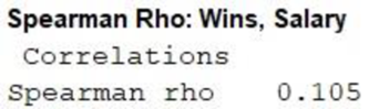
Thus, the rank correlation coefficient between the number of Wins and team salary is 0.105.
Denote the population correlation as
The null and alternative hypotheses are stated as follows:
Null hypothesis:
That is, the correlation between the ranks of the number of wins and team salary.
Alternative hypothesis:
That is, there is positive correlation in the ranks of the number of wins and team salary.
Test statistic:
The test statistic is as follows:
Here, sample size is 30 and correlation coefficient is 0.105.
The test statistic is computed as follows:
Thus, the test statistic value is 0.559.
Degrees of freedom:
The level of significance is 0.01.
Step-by-step software procedure to obtain the critical value using EXCEL software is as follows:
- Open an EXCEL file.
- In cell A1, enter the formula “=T.INV (0.01, 12)”.
Output using the EXCEL is given as follows:

From the EXCEL output, the critical value for the right tailed test is 2.467
Decision rule:
Reject the null hypothesis H0 if,
Otherwise fail to reject H0.
Conclusion:
The value of test statistic is 0.559 and critical value is 2.467.
Here,
By the rejection rule, fail to reject the null hypothesis at the 0.01 significance level.
Thus, there is no sufficient evidence to conclude that there is a positive correlation in the ranks of the number of wins and team salary.
b.
Conduct a test of hypothesis to see whether there is a difference in the distribution of team salaries for the American League and National League.
Answer to Problem 42DE
There is no difference in the distributions of the team salaries for the American League and National League.
Explanation of Solution
The Mann-Whitney test is suitable for the comparison of two inpendent groups.
The null and alternative hypotheses are stated as follows:
Null hypothesis: There is no difference in the distributions of the team salaries for the American League and National League.
Alternative hypothesis: There is a difference in the distributions of the team salaries for the American League and National League.
Step-by-step procedure to obtain the test statistic using Excel MegaStat software is as follows:
- Choose MegaStat > Nonparametric Tests > Wilcoxon – Mann/Whitney Test.
- In Group 1, enter the column of American League.
- In Group 2, enter the second column of National League.
- Select on Continuity correction and Select the Alternative.
- Click OK
Output obtained using Excel Mega stat software is as follows:
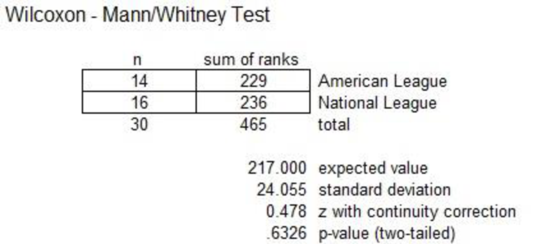
From the above output, the value of the test statistic is 0.478 and the p-value is 0.6326.
Conclusion:
Consider the significance level is 0.05.
Here, the p-value is greater than the significance level 0.05.
By the rejection rule, fail to reject the null hypothesis at the 0.05 significance level.
Therefore, there is no difference in the distributions of the team salaries for the American League and National League.
c.
Find the coefficient of rank correlation between attendance and team salary.
Check whether it is reasonable to conclude the ranks of these two variables are related.
Answer to Problem 42DE
The coefficient of rank correlation between attendance and team salary is 0.805.
Explanation of Solution
Step-by-step procedure to obtain the rank correlation using Minitab software:
- Select Stat > Basic Statistics > Correlation.
- In Variables, select Attendance, and team salary from the box on the left.
- Click OK.
Output obtained using Minitab is as follows:

From the above output, the coefficient of rank correlation between attendance and team salary is 0.805.
Denote the population correlation as
The null and alternative hypotheses are stated below:
Null hypothesis:
That is, there is no correlation between attendance and team salary.
Alternative hypothesis:
That is, there is a correlation between attendance and team salary.
Here, sample size is 30 and correlation coefficient is 0.805.
The test statistic is as follows:
Thus, the test statistic value is 7.18.
Degrees of freedom:
The level of significance is 0.05.
Step-by-step software procedure to obtain the critical value using EXCEL software is as follows:
- Open an EXCEL file.
- In cell A1, enter the formula “=T.INV.2T (0.05, 28)”.
Output using the EXCEL is given as follows:
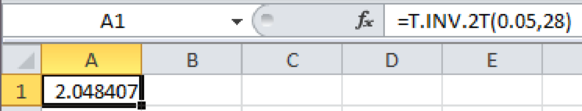
From the EXCEL output, the critical value is 2.048
Conclusion:
The value of test statistic is 7.18 and critical value is 2.048.
Here,
By the rejection rule, reject the null hypothesis at the 0.05 significance level.
Therefore, it is reasonable to conclude that the ranks of these two variables are related.
Want to see more full solutions like this?
Chapter 16 Solutions
Statistical Techniques in Business and Economics, 16th Edition


- Examine the Variables: Carefully review and note the names of all variables in the dataset. Examples of these variables include: Mileage (mpg) Number of Cylinders (cyl) Displacement (disp) Horsepower (hp) Research: Google to understand these variables. Statistical Analysis: Select mpg variable, and perform the following statistical tests. Once you are done with these tests using mpg variable, repeat the same with hp Mean Median First Quartile (Q1) Second Quartile (Q2) Third Quartile (Q3) Fourth Quartile (Q4) 10th Percentile 70th Percentile Skewness Kurtosis Document Your Results: In RStudio: Before running each statistical test, provide a heading in the format shown at the bottom. “# Mean of mileage – Your name’s command” In Microsoft Word: Once you've completed all tests, take a screenshot of your results in RStudio and paste it into a Microsoft Word document. Make sure that snapshots are very clear. You will need multiple snapshots. Also transfer these results to the…arrow_forward2 (VaR and ES) Suppose X1 are independent. Prove that ~ Unif[-0.5, 0.5] and X2 VaRa (X1X2) < VaRa(X1) + VaRa (X2). ~ Unif[-0.5, 0.5]arrow_forward8 (Correlation and Diversification) Assume we have two stocks, A and B, show that a particular combination of the two stocks produce a risk-free portfolio when the correlation between the return of A and B is -1.arrow_forward
- 9 (Portfolio allocation) Suppose R₁ and R2 are returns of 2 assets and with expected return and variance respectively r₁ and 72 and variance-covariance σ2, 0%½ and σ12. Find −∞ ≤ w ≤ ∞ such that the portfolio wR₁ + (1 - w) R₂ has the smallest risk.arrow_forward7 (Multivariate random variable) Suppose X, €1, €2, €3 are IID N(0, 1) and Y2 Y₁ = 0.2 0.8X + €1, Y₂ = 0.3 +0.7X+ €2, Y3 = 0.2 + 0.9X + €3. = (In models like this, X is called the common factors of Y₁, Y₂, Y3.) Y = (Y1, Y2, Y3). (a) Find E(Y) and cov(Y). (b) What can you observe from cov(Y). Writearrow_forward1 (VaR and ES) Suppose X ~ f(x) with 1+x, if 0> x > −1 f(x) = 1−x if 1 x > 0 Find VaRo.05 (X) and ES0.05 (X).arrow_forward
- Joy is making Christmas gifts. She has 6 1/12 feet of yarn and will need 4 1/4 to complete our project. How much yarn will she have left over compute this solution in two different ways arrow_forwardSolve for X. Explain each step. 2^2x • 2^-4=8arrow_forwardOne hundred people were surveyed, and one question pertained to their educational background. The results of this question and their genders are given in the following table. Female (F) Male (F′) Total College degree (D) 30 20 50 No college degree (D′) 30 20 50 Total 60 40 100 If a person is selected at random from those surveyed, find the probability of each of the following events.1. The person is female or has a college degree. Answer: equation editor Equation Editor 2. The person is male or does not have a college degree. Answer: equation editor Equation Editor 3. The person is female or does not have a college degree.arrow_forward
 Glencoe Algebra 1, Student Edition, 9780079039897...AlgebraISBN:9780079039897Author:CarterPublisher:McGraw Hill
 Holt Mcdougal Larson Pre-algebra: Student Edition...AlgebraISBN:9780547587776Author:HOLT MCDOUGALPublisher:HOLT MCDOUGAL
 Big Ideas Math A Bridge To Success Algebra 1: Stu...AlgebraISBN:9781680331141Author:HOUGHTON MIFFLIN HARCOURTPublisher:Houghton Mifflin Harcourt