Videos
State the hypotheses, test statistic and the two-tailed p-value.
Make a decision for the research question “whether there is significant
Identify the issues of
Identify whether non-normality is concerned or not.
Answer to Problem 36CE
The hypotheses for the test are given below:
Null hypothesis:
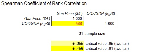
The rank correlation between gasoline price and carbon dioxide emission is zero.
Alternate Hypothesis:
The rank correlation between gasoline price and carbon dioxide is greater than zero.
The test statistic and the p-value are –0.588 and 0.355 respectively.
There is a support evidence to conclude that there exists a significant correlation between gasoline price and carbon dioxide emission at 5% level of significance.
The decision is close since the rejection of null hypothesis is close to the research question “whether there is significant correlation between gasoline price and carbon dioxide emission?”
The sample size is not an issue.
The gasoline price follows normality but the carbon dioxide emission does not follow normality.
Explanation of Solution
Calculation:
The given information is that, the data shows gasoline price and carbon emissions for selected nations. The level of significance is 0.05.
The hypotheses for the test are given below:
Null hypothesis:
The rank correlation between gasoline price and carbon dioxide emission is zero.
Alternate Hypothesis:
The rank correlation between gasoline price and carbon dioxide emission is greater than zero.
Software procedure:
Step-by-step procedure to find the
- Choose MegaStat > Nonparametric Tests > Spearman Coefficient of Rank Correlation.
- In Input
range , select the cells A1:B32. - Unselect Output ranked data and Correct for ties.
- Click OK.
Output obtained from MegaStat is given below:
Decision Rule:
Reject the null hypothesis
Conclusion:
The absolute value of the test statistic is 0.588 and the critical value for the desired level of significance
The test statistic is greater than the critical value.
That is,
Thus, the null hypothesis is rejected.
Hence, there is a support of evidence to conclude that there exists a significant correlation between gasoline price and carbon dioxide at 5% level of significance.
Histogram for gasoline price:
Step-by-step procedure to construct a histogram using MINITAB is given below:
- Choose Basic Statistics > Graphical Summary.
- Choose Simple, and then click OK.
- In variables, enter the column of Gasoline price.
- In Confidence level, enter 95.0.
- Click OK.
Output obtained from MINITAB is given below:
Interpretation:
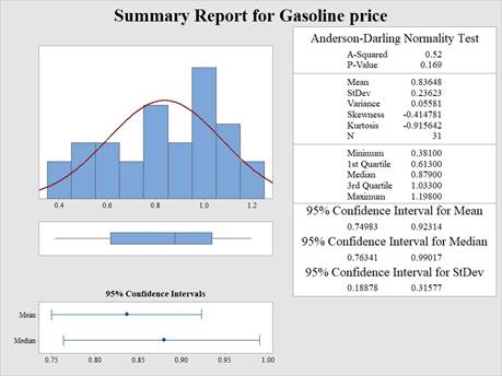
The histogram appears to be left skewed since the tail is elongated towards the left than to the right side. Hence, the test of normality is recommended.
Testing the normality using Anderson Darling test:
Null hypothesis:
Alternate Hypothesis:
Decision Rule:
Reject the null hypothesis
Conclusion:
The p-value for the A-D test is 0.169 and the level of significance is 0.05.
The p-value for the A-D test is greater than the level of significance.
That is,
Thus, the null hypothesis is rejected.
Hence, there is a support of evidence to assume that gasoline follows normal distribution at 5% level of significance.
Histogram for carbon dioxide emission:
Step-by-step procedure to construct a histogram using MINITAB is given below:
- Choose Basic Statistics > Graphical Summary.
- Choose Simple, and then click OK.
- In variables, enter the column of carbon dioxide emission.
- In Confidence level, enter 95.0.
- Click OK.
Output obtained from MINITAB is given below:
Interpretation:
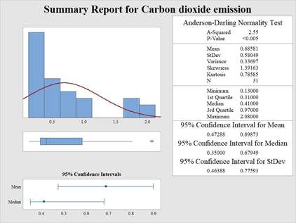
The histogram appears to be right skewed since the tail is elongated towards the right than to the left side. Hence, the test of normality is recommended.
Testing the normality using Anderson Darling test:
Null hypothesis:
Alternate Hypothesis:
Decision Rule:
Reject the null hypothesis
Conclusion:
The p-value for the A-D test is lesser than 0.005 and the level of significance is 0.05.
The p-value for the A-D test is lesser than the level of significance.
That is,
Thus, the null hypothesis is rejected.
Hence, there is no support of evidence to assume that the carbon dioxide emission follows normal distribution at 5% level of significance.
Want to see more full solutions like this?
Chapter 16 Solutions
APPLIED STAT.IN BUS.+ECONOMICS


- The details of the clock sales at a supermarket for the past 6 weeks are shown in the table below. The time series appears to be relatively stable, without trend, seasonal, or cyclical effects. The simple moving average value of k is set at 2. Calculate the value of the simple moving average mean absolute percentage error. Round to two decimal places. Week Units sold 1 88 2 44 3 54 4 65 5 72 6 85 Part 1 A. 14.39 B. 25.56 C. 23.45 D. 20.90arrow_forwardThe accompanying data shows the fossil fuels production, fossil fuels consumption, and total energy consumption in quadrillions of BTUs of a certain region for the years 1986 to 2015. Complete parts a and b. Year Fossil Fuels Production Fossil Fuels Consumption Total Energy Consumption1949 28.748 29.002 31.9821950 32.563 31.632 34.6161951 35.792 34.008 36.9741952 34.977 33.800 36.7481953 35.349 34.826 37.6641954 33.764 33.877 36.6391955 37.364 37.410 40.2081956 39.771 38.888 41.7541957 40.133 38.926 41.7871958 37.216 38.717 41.6451959 39.045 40.550 43.4661960 39.869 42.137 45.0861961 40.307 42.758 45.7381962 41.732 44.681 47.8261963 44.037 46.509 49.6441964 45.789 48.543 51.8151965 47.235 50.577 54.0151966 50.035 53.514 57.0141967 52.597 55.127 58.9051968 54.306 58.502 62.4151969 56.286…arrow_forwardThe accompanying data shows the fossil fuels production, fossil fuels consumption, and total energy consumption in quadrillions of BTUs of a certain region for the years 1986 to 2015. Complete parts a and b. Year Fossil Fuels Production Fossil Fuels Consumption Total Energy Consumption1949 28.748 29.002 31.9821950 32.563 31.632 34.6161951 35.792 34.008 36.9741952 34.977 33.800 36.7481953 35.349 34.826 37.6641954 33.764 33.877 36.6391955 37.364 37.410 40.2081956 39.771 38.888 41.7541957 40.133 38.926 41.7871958 37.216 38.717 41.6451959 39.045 40.550 43.4661960 39.869 42.137 45.0861961 40.307 42.758 45.7381962 41.732 44.681 47.8261963 44.037 46.509 49.6441964 45.789 48.543 51.8151965 47.235 50.577 54.0151966 50.035 53.514 57.0141967 52.597 55.127 58.9051968 54.306 58.502 62.4151969 56.286…arrow_forward
- The accompanying data shows the fossil fuels production, fossil fuels consumption, and total energy consumption in quadrillions of BTUs of a certain region for the years 1986 to 2015. Complete parts a and b. Develop line charts for each variable and identify the characteristics of the time series (that is, random, stationary, trend, seasonal, or cyclical). What is the line chart for the variable Fossil Fuels Production?arrow_forwardThe accompanying data shows the fossil fuels production, fossil fuels consumption, and total energy consumption in quadrillions of BTUs of a certain region for the years 1986 to 2015. Complete parts a and b. Year Fossil Fuels Production Fossil Fuels Consumption Total Energy Consumption1949 28.748 29.002 31.9821950 32.563 31.632 34.6161951 35.792 34.008 36.9741952 34.977 33.800 36.7481953 35.349 34.826 37.6641954 33.764 33.877 36.6391955 37.364 37.410 40.2081956 39.771 38.888 41.7541957 40.133 38.926 41.7871958 37.216 38.717 41.6451959 39.045 40.550 43.4661960 39.869 42.137 45.0861961 40.307 42.758 45.7381962 41.732 44.681 47.8261963 44.037 46.509 49.6441964 45.789 48.543 51.8151965 47.235 50.577 54.0151966 50.035 53.514 57.0141967 52.597 55.127 58.9051968 54.306 58.502 62.4151969 56.286…arrow_forwardFor each of the time series, construct a line chart of the data and identify the characteristics of the time series (that is, random, stationary, trend, seasonal, or cyclical). Month PercentApr 1972 4.97May 1972 5.00Jun 1972 5.04Jul 1972 5.25Aug 1972 5.27Sep 1972 5.50Oct 1972 5.73Nov 1972 5.75Dec 1972 5.79Jan 1973 6.00Feb 1973 6.02Mar 1973 6.30Apr 1973 6.61May 1973 7.01Jun 1973 7.49Jul 1973 8.30Aug 1973 9.23Sep 1973 9.86Oct 1973 9.94Nov 1973 9.75Dec 1973 9.75Jan 1974 9.73Feb 1974 9.21Mar 1974 8.85Apr 1974 10.02May 1974 11.25Jun 1974 11.54Jul 1974 11.97Aug 1974 12.00Sep 1974 12.00Oct 1974 11.68Nov 1974 10.83Dec 1974 10.50Jan 1975 10.05Feb 1975 8.96Mar 1975 7.93Apr 1975 7.50May 1975 7.40Jun 1975 7.07Jul 1975 7.15Aug 1975 7.66Sep 1975 7.88Oct 1975 7.96Nov 1975 7.53Dec 1975 7.26Jan 1976 7.00Feb 1976 6.75Mar 1976 6.75Apr 1976 6.75May 1976…arrow_forward
- Hi, I need to make sure I have drafted a thorough analysis, so please answer the following questions. Based on the data in the attached image, develop a regression model to forecast the average sales of football magazines for each of the seven home games in the upcoming season (Year 10). That is, you should construct a single regression model and use it to estimate the average demand for the seven home games in Year 10. In addition to the variables provided, you may create new variables based on these variables or based on observations of your analysis. Be sure to provide a thorough analysis of your final model (residual diagnostics) and provide assessments of its accuracy. What insights are available based on your regression model?arrow_forwardI want to make sure that I included all possible variables and observations. There is a considerable amount of data in the images below, but not all of it may be useful for your purposes. Are there variables contained in the file that you would exclude from a forecast model to determine football magazine sales in Year 10? If so, why? Are there particular observations of football magazine sales from previous years that you would exclude from your forecasting model? If so, why?arrow_forwardStat questionsarrow_forward
- 1) and let Xt is stochastic process with WSS and Rxlt t+t) 1) E (X5) = \ 1 2 Show that E (X5 = X 3 = 2 (= = =) Since X is WSSEL 2 3) find E(X5+ X3)² 4) sind E(X5+X2) J=1 ***arrow_forwardProve that 1) | RxX (T) | << = (R₁ " + R$) 2) find Laplalse trans. of Normal dis: 3) Prove thy t /Rx (z) | < | Rx (0)\ 4) show that evary algebra is algebra or not.arrow_forwardFor each of the time series, construct a line chart of the data and identify the characteristics of the time series (that is, random, stationary, trend, seasonal, or cyclical). Month Number (Thousands)Dec 1991 65.60Jan 1992 71.60Feb 1992 78.80Mar 1992 111.60Apr 1992 107.60May 1992 115.20Jun 1992 117.80Jul 1992 106.20Aug 1992 109.90Sep 1992 106.00Oct 1992 111.80Nov 1992 84.50Dec 1992 78.60Jan 1993 70.50Feb 1993 74.60Mar 1993 95.50Apr 1993 117.80May 1993 120.90Jun 1993 128.50Jul 1993 115.30Aug 1993 121.80Sep 1993 118.50Oct 1993 123.30Nov 1993 102.30Dec 1993 98.70Jan 1994 76.20Feb 1994 83.50Mar 1994 134.30Apr 1994 137.60May 1994 148.80Jun 1994 136.40Jul 1994 127.80Aug 1994 139.80Sep 1994 130.10Oct 1994 130.60Nov 1994 113.40Dec 1994 98.50Jan 1995 84.50Feb 1995 81.60Mar 1995 103.80Apr 1995 116.90May 1995 130.50Jun 1995 123.40Jul 1995 129.10Aug 1995…arrow_forward
 Glencoe Algebra 1, Student Edition, 9780079039897...AlgebraISBN:9780079039897Author:CarterPublisher:McGraw Hill
 Holt Mcdougal Larson Pre-algebra: Student Edition...AlgebraISBN:9780547587776Author:HOLT MCDOUGALPublisher:HOLT MCDOUGAL
 Big Ideas Math A Bridge To Success Algebra 1: Stu...AlgebraISBN:9781680331141Author:HOUGHTON MIFFLIN HARCOURTPublisher:Houghton Mifflin Harcourt
 Algebra: Structure And Method, Book 1AlgebraISBN:9780395977224Author:Richard G. Brown, Mary P. Dolciani, Robert H. Sorgenfrey, William L. ColePublisher:McDougal Littell