Videos
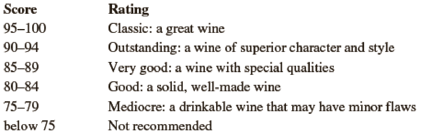
Wine Spectator magazine contains articles and reviews on every aspect of the wine industry, including ratings of wine from around the world. In a recent issue they reviewed and scored 475 wines from the Piedmont region of Italy using a 100-point scale. The following table shows how the Wine Spectator score each wine received is used to rate each wine as being classic, outstanding, very good, good, mediocre, or not recommended.
A key question for most consumers is whether paying more for a bottle of wine will result in a better wine. To investigate this question for wines from the Piedmont region we selected a random sample of 100 of the 475 wines that Wine Spectator reviewed. The data, contained in the DATAfile named WineRatings, shows the price ($), the Wine Spectator score, and the rating for each wine.
Managerial Report
- 1. Develop a table that shows the number of wines that were classified as classic, outstanding, very good, good, mediocre, and not recommended and the average price. Does there appear to be any relationship between the price of the wine and the Wine Spectator rating? Are there any other aspects of your initial summary of the data that stand out?
- 2. Develop a
scatter diagram with price on the horizontal axis and the Wine Spectator score on the vertical axis. Does the relationship between price and score appear to be linear? - 3. Using linear regression, develop an estimated regression equation that can be used to predict the score given the price of the wine.
- 4. Using a second-order model, develop an estimated regression equation that can be used to predict the score given the price of the wine.
- 5. Compare the results from fitting a linear model and fitting a second-order model.
- 6. As an alternative to fitting a second-order model, fit a model using the natural logarithm of price as the independent variable. Compare the results with the second-order model.
- 7. Based upon your analysis, would you say that spending more for a bottle of wine will provide a better wine?
- 8. Suppose that you want to spend a maximum of $30 for a bottle of wine. In this case, will spending closer to your upper limit for price result in a better wine than a much lower price?

Trending nowThis is a popular solution!

Chapter 16 Solutions
Modern Business Statistics with Microsoft Office Excel (with XLSTAT Education Edition Printed Access Card) (MindTap Course List)


- Compute the relative risk of falling for the two groups (did not stop walking vs. did stop). State/interpret your result verbally.arrow_forwardMicrosoft Excel include formulasarrow_forwardQuestion 1 The data shown in Table 1 are and R values for 24 samples of size n = 5 taken from a process producing bearings. The measurements are made on the inside diameter of the bearing, with only the last three decimals recorded (i.e., 34.5 should be 0.50345). Table 1: Bearing Diameter Data Sample Number I R Sample Number I R 1 34.5 3 13 35.4 8 2 34.2 4 14 34.0 6 3 31.6 4 15 37.1 5 4 31.5 4 16 34.9 7 5 35.0 5 17 33.5 4 6 34.1 6 18 31.7 3 7 32.6 4 19 34.0 8 8 33.8 3 20 35.1 9 34.8 7 21 33.7 2 10 33.6 8 22 32.8 1 11 31.9 3 23 33.5 3 12 38.6 9 24 34.2 2 (a) Set up and R charts on this process. Does the process seem to be in statistical control? If necessary, revise the trial control limits. [15 pts] (b) If specifications on this diameter are 0.5030±0.0010, find the percentage of nonconforming bearings pro- duced by this process. Assume that diameter is normally distributed. [10 pts] 1arrow_forward
- 4. (5 pts) Conduct a chi-square contingency test (test of independence) to assess whether there is an association between the behavior of the elderly person (did not stop to talk, did stop to talk) and their likelihood of falling. Below, please state your null and alternative hypotheses, calculate your expected values and write them in the table, compute the test statistic, test the null by comparing your test statistic to the critical value in Table A (p. 713-714) of your textbook and/or estimating the P-value, and provide your conclusions in written form. Make sure to show your work. Did not stop walking to talk Stopped walking to talk Suffered a fall 12 11 Totals 23 Did not suffer a fall | 2 Totals 35 37 14 46 60 Tarrow_forwardQuestion 2 Parts manufactured by an injection molding process are subjected to a compressive strength test. Twenty samples of five parts each are collected, and the compressive strengths (in psi) are shown in Table 2. Table 2: Strength Data for Question 2 Sample Number x1 x2 23 x4 x5 R 1 83.0 2 88.6 78.3 78.8 3 85.7 75.8 84.3 81.2 78.7 75.7 77.0 71.0 84.2 81.0 79.1 7.3 80.2 17.6 75.2 80.4 10.4 4 80.8 74.4 82.5 74.1 75.7 77.5 8.4 5 83.4 78.4 82.6 78.2 78.9 80.3 5.2 File Preview 6 75.3 79.9 87.3 89.7 81.8 82.8 14.5 7 74.5 78.0 80.8 73.4 79.7 77.3 7.4 8 79.2 84.4 81.5 86.0 74.5 81.1 11.4 9 80.5 86.2 76.2 64.1 80.2 81.4 9.9 10 75.7 75.2 71.1 82.1 74.3 75.7 10.9 11 80.0 81.5 78.4 73.8 78.1 78.4 7.7 12 80.6 81.8 79.3 73.8 81.7 79.4 8.0 13 82.7 81.3 79.1 82.0 79.5 80.9 3.6 14 79.2 74.9 78.6 77.7 75.3 77.1 4.3 15 85.5 82.1 82.8 73.4 71.7 79.1 13.8 16 78.8 79.6 80.2 79.1 80.8 79.7 2.0 17 82.1 78.2 18 84.5 76.9 75.5 83.5 81.2 19 79.0 77.8 20 84.5 73.1 78.2 82.1 79.2 81.1 7.6 81.2 84.4 81.6 80.8…arrow_forwardName: Lab Time: Quiz 7 & 8 (Take Home) - due Wednesday, Feb. 26 Contingency Analysis (Ch. 9) In lab 5, part 3, you will create a mosaic plot and conducted a chi-square contingency test to evaluate whether elderly patients who did not stop walking to talk (vs. those who did stop) were more likely to suffer a fall in the next six months. I have tabulated the data below. Answer the questions below. Please show your calculations on this or a separate sheet. Did not stop walking to talk Stopped walking to talk Totals Suffered a fall Did not suffer a fall Totals 12 11 23 2 35 37 14 14 46 60 Quiz 7: 1. (2 pts) Compute the odds of falling for each group. Compute the odds ratio for those who did not stop walking vs. those who did stop walking. Interpret your result verbally.arrow_forward
- Solve please and thank you!arrow_forward7. In a 2011 article, M. Radelet and G. Pierce reported a logistic prediction equation for the death penalty verdicts in North Carolina. Let Y denote whether a subject convicted of murder received the death penalty (1=yes), for the defendant's race h (h1, black; h = 2, white), victim's race i (i = 1, black; i = 2, white), and number of additional factors j (j = 0, 1, 2). For the model logit[P(Y = 1)] = a + ß₁₂ + By + B²², they reported = -5.26, D â BD = 0, BD = 0.17, BY = 0, BY = 0.91, B = 0, B = 2.02, B = 3.98. (a) Estimate the probability of receiving the death penalty for the group most likely to receive it. [4 pts] (b) If, instead, parameters used constraints 3D = BY = 35 = 0, report the esti- mates. [3 pts] h (c) If, instead, parameters used constraints Σ₁ = Σ₁ BY = Σ; B = 0, report the estimates. [3 pts] Hint the probabilities, odds and odds ratios do not change with constraints.arrow_forwardSolve please and thank you!arrow_forward
- Solve please and thank you!arrow_forwardQuestion 1:We want to evaluate the impact on the monetary economy for a company of two types of strategy (competitive strategy, cooperative strategy) adopted by buyers.Competitive strategy: strategy characterized by firm behavior aimed at obtaining concessions from the buyer.Cooperative strategy: a strategy based on a problem-solving negotiating attitude, with a high level of trust and cooperation.A random sample of 17 buyers took part in a negotiation experiment in which 9 buyers adopted the competitive strategy, and the other 8 the cooperative strategy. The savings obtained for each group of buyers are presented in the pdf that i sent: For this problem, we assume that the samples are random and come from two normal populations of unknown but equal variances.According to the theory, the average saving of buyers adopting a competitive strategy will be lower than that of buyers adopting a cooperative strategy.a) Specify the population identifications and the hypotheses H0 and H1…arrow_forwardYou assume that the annual incomes for certain workers are normal with a mean of $28,500 and a standard deviation of $2,400. What’s the chance that a randomly selected employee makes more than $30,000?What’s the chance that 36 randomly selected employees make more than $30,000, on average?arrow_forward
 Big Ideas Math A Bridge To Success Algebra 1: Stu...AlgebraISBN:9781680331141Author:HOUGHTON MIFFLIN HARCOURTPublisher:Houghton Mifflin Harcourt
 Glencoe Algebra 1, Student Edition, 9780079039897...AlgebraISBN:9780079039897Author:CarterPublisher:McGraw Hill
 Holt Mcdougal Larson Pre-algebra: Student Edition...AlgebraISBN:9780547587776Author:HOLT MCDOUGALPublisher:HOLT MCDOUGAL