Concept explainers
Videos
(a)
Complete the F table.
Make a decision to retain or reject the null hypothesis that the multiple regression equation can be used to significantly predict health.
(a)
Answer to Problem 28CAP
The completed F table is,
| Source of variation | SS | df | MS | |
| Regression | 126.22 | 2 | 63.11 | 14.48 |
| Residual (error) | 21.78 | 5 | 4.36 | |
| Total | 148.00 | 7 |
The decision is to reject the null hypothesis.
Theregression equation significantly predicts variance in criterion variable (Y) health [BMI].
Explanation of Solution
Calculation:
The given information is that, the researcher has tested whether ‘daily intake of fat (in grams)’ and ‘amount of exercise (in minutes)’ can predict health (measured using a body mass index [BMI] scale.
The formula for test statistic is,
Decision rules:
- If the test statistic value is greater than the critical value, then reject the null hypothesis
- If the test statistic value is smaller than the critical value, then retain the null hypothesis
Null hypothesis:
Alternative hypothesis:
Software procedure:
Step by step procedure to obtain test statistic value using SPSS software is given as,
- Choose Variable view.
- Under the name, enter the name as Fat, Exercise, Health.
- Choose Data view, enter the data.
- Choose Analyze>Regression>Linear.
- In Dependents, enter the column of Health.
- In Independents, enter the column of Fat, and Exercise.
- Click OK.
Output using SPSS software is given below:
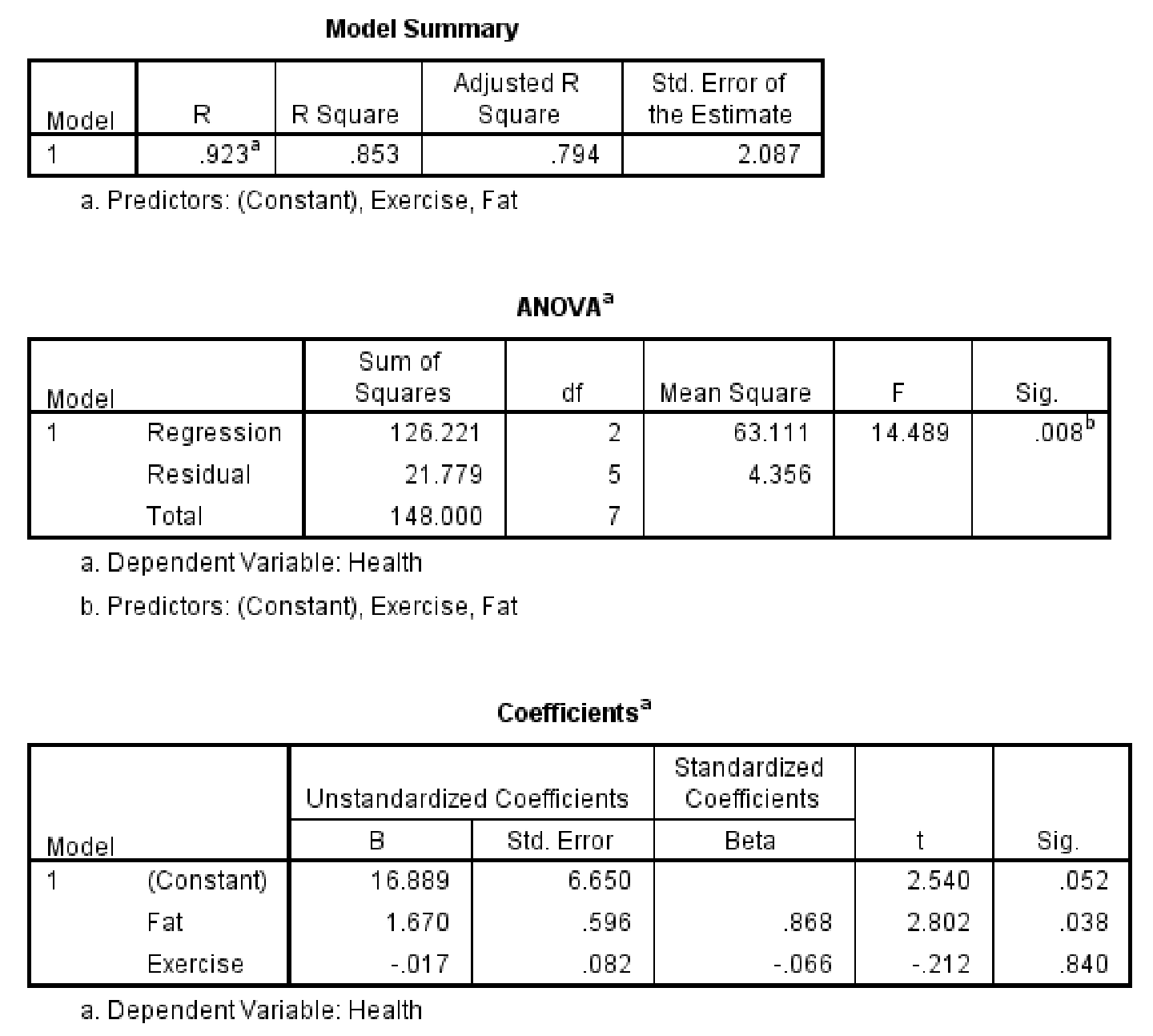
The table of F is,
| Source of variation | SS | df | MS | |
| Regression | 126.22 | 2 | 63.11 | 14.48 |
| Residual (error) | 21.78 | 5 | 4.36 | |
| Total | 148.00 | 7 |
Table 1
Critical value:
The considered significance level is
The degrees of freedom for regression are 2, the degrees of freedom for residual are 5.
From the Appendix B: Table B.3-Critical values for F distribution:
- Locate the value 2 in degrees of freedomnumerator row.
- Locate the value 5 in degrees of freedomdenominator row.
- Locate the 0.05 level of significance (value in lightface type) in combined row.
- The intersecting value that corresponds to the (2, 5) with level of significance 0.05 is 5.79.
Thus, the critical value for
Conclusion:
The value of test statistic is 14.48.
The critical value is 5.79.
The test statistic value is greater than the critical value.
The test statistic value falls under critical region.
Hence the null hypothesis is rejected.
Thus, the regression equation significantly predicts variance in criterion variable (Y) health [BMI].
(b)
Determine which predictor variable or variables, when added to the multiple regression equation, significantly contributed to predictions in Y (health).
(b)
Answer to Problem 28CAP
The predictor variable daily intake of fat significantly contributed to predictions in Y (health) when added to the multiple regression equation.
Explanation of Solution
Calculation:
The given information is that, a sample of 8 scores is recorded. The predictor variables are ‘daily intake of fat (in grams)
Relative contribution to fat
Null hypothesis:
Alternative hypothesis:
The predictor variable fat is tested. The other predictor variable that is not tested is ‘Exercise’. Calculate the correlation between ‘Exercise’ and ‘Health[BMI]’.
Software procedure:
Step by step procedure to obtain correlation using SPSS software is given as,
- Choose Variable view.
- Under the name, enter the name as Health, Exercise.
- Choose Data view, enter the data.
- Choose Analyze>Correlate>Bivariate.
- In variables, enter the Health, and Exercise.
- Click OK.
Output using SPSS software is given below:
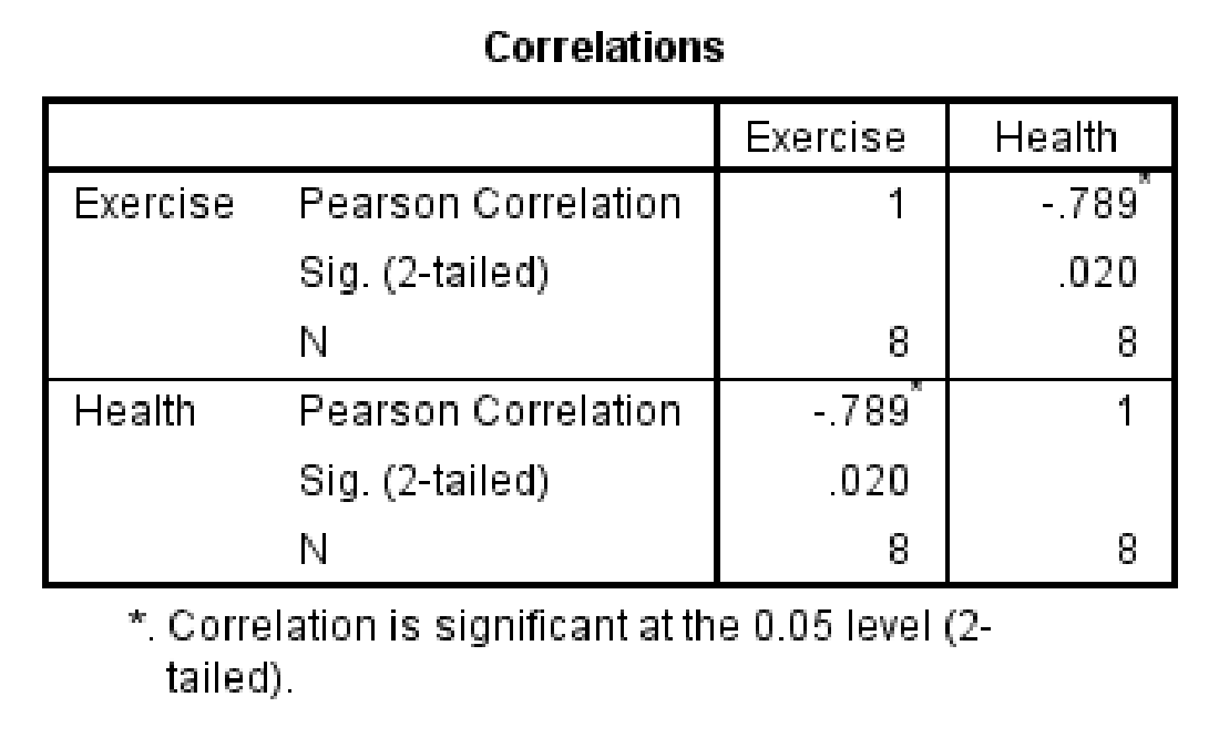
The correlation between ‘Exercise’ and ‘Health [BMI]’ is –0.789.
The value of
The formula for
The calculation of sums of squares is,
|
Health [BMI] (Y) | |
| 32 | 1,024 |
| 34 | 1,156 |
| 23 | 529 |
| 33 | 1,089 |
| 28 | 784 |
| 27 | 729 |
| 25 | 625 |
| 22 | 484 |
Table 2
Substitute,
The contribution of
From the F table, the value of
The contribution of
Reproduce the F table by replacing,
Since there would be only one predictor variable, the degrees of freedom for regression would be 1.
The mean sums of squares for regression is,
The F statistic value is,
The change F table with
| Source of variation | SS | df | MS | |
| Regression | 34.09 | 1 | 34.09 | 7.82 |
| Residual (error) | 21.78 | 5 | 4.36 | |
| Total | 148.00 | 7 |
Critical value:
The considered significance level is
The degrees of freedom for regression are 1, the degrees of freedom for residual are 5.
From the Appendix B: Table B.3-Critical values for F distribution:
- Locate the value 1 in degrees of freedom numerator row.
- Locate the value 5 in degrees of freedom denominator row.
- Locate the 0.05 level of significance (value in lightface type) in combined row.
- The intersecting value that corresponds to the (1, 5) with level of significance 0.05 is 6.61.
Thus, the critical value for
Conclusion:
The value of test statistic is 7.82.
The critical value is 6.61.
The test statistic value is greater than the critical value.
The test statistic value falls under critical region.
Hence the null hypothesis is rejected.
Thus, adding fat
Relative contribution to exercise
Null hypothesis:
Alternative hypothesis:
The predictor variable exercise is tested. The other predictor variable that is not tested is ‘fat’. Calculate the correlation between ‘fat’ and ‘Health [BMI]’.
Software procedure:
Step by step procedure to obtain correlation using SPSS software is given as,
- Choose Variable view.
- Under the name, enter the name as Health, Fat.
- Choose Data view, enter the data.
- Choose Analyze>Correlate>Bivariate.
- In variables, enter the Health, and Fat.
- Click OK.
Output using SPSS software is given below:
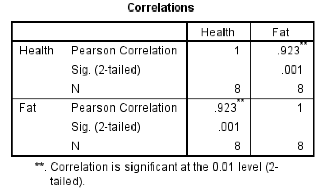
The correlation between ‘fat’ and ‘Health [BMI]’ is 0.923.
The value of
The value for
From the F table, the value of
The contribution of
Reproduce the F table by replacing,
Since there would be only one predictor variable, the degrees of freedom for regression would be 1.
The mean sums of squares for regression is,
The F statistic value is,
The change F table with
| Source of variation | SS | df | MS | |
| Regression | 0.14 | 1 | 0.14 | 0.03 |
| Residual (error) | 21.78 | 5 | 4.36 | |
| Total | 148.00 | 7 |
The critical value for F table with
Conclusion:
The value of test statistic is 0.03.
The critical value is 6.61.
The test statistic value is less than the critical value.
The test statistic value does not fall under critical region.
Hence the null hypothesis is retained.
Thus, adding exercise
Hence, the predictor variable daily intake of fat significantly contributed to predictions in Y (health) when added to the multiple regression equation.
Want to see more full solutions like this?
Chapter 16 Solutions
Statistics for the Behavioral Sciences


- Client 1 Weight before diet (pounds) Weight after diet (pounds) 128 120 2 131 123 3 140 141 4 178 170 5 121 118 6 136 136 7 118 121 8 136 127arrow_forwardClient 1 Weight before diet (pounds) Weight after diet (pounds) 128 120 2 131 123 3 140 141 4 178 170 5 121 118 6 136 136 7 118 121 8 136 127 a) Determine the mean change in patient weight from before to after the diet (after – before). What is the 95% confidence interval of this mean difference?arrow_forwardIn order to find probability, you can use this formula in Microsoft Excel: The best way to understand and solve these problems is by first drawing a bell curve and marking key points such as x, the mean, and the areas of interest. Once marked on the bell curve, figure out what calculations are needed to find the area of interest. =NORM.DIST(x, Mean, Standard Dev., TRUE). When the question mentions “greater than” you may have to subtract your answer from 1. When the question mentions “between (two values)”, you need to do separate calculation for both values and then subtract their results to get the answer. 1. Compute the probability of a value between 44.0 and 55.0. (The question requires finding probability value between 44 and 55. Solve it in 3 steps. In the first step, use the above formula and x = 44, calculate probability value. In the second step repeat the first step with the only difference that x=55. In the third step, subtract the answer of the first part from the…arrow_forward
- If a uniform distribution is defined over the interval from 6 to 10, then answer the followings: What is the mean of this uniform distribution? Show that the probability of any value between 6 and 10 is equal to 1.0 Find the probability of a value more than 7. Find the probability of a value between 7 and 9. The closing price of Schnur Sporting Goods Inc. common stock is uniformly distributed between $20 and $30 per share. What is the probability that the stock price will be: More than $27? Less than or equal to $24? The April rainfall in Flagstaff, Arizona, follows a uniform distribution between 0.5 and 3.00 inches. What is the mean amount of rainfall for the month? What is the probability of less than an inch of rain for the month? What is the probability of exactly 1.00 inch of rain? What is the probability of more than 1.50 inches of rain for the month? The best way to solve this problem is begin by creating a chart. Clearly mark the range, identifying the lower and upper…arrow_forwardProblem 1: The mean hourly pay of an American Airlines flight attendant is normally distributed with a mean of 40 per hour and a standard deviation of 3.00 per hour. What is the probability that the hourly pay of a randomly selected flight attendant is: Between the mean and $45 per hour? More than $45 per hour? Less than $32 per hour? Problem 2: The mean of a normal probability distribution is 400 pounds. The standard deviation is 10 pounds. What is the area between 415 pounds and the mean of 400 pounds? What is the area between the mean and 395 pounds? What is the probability of randomly selecting a value less than 395 pounds? Problem 3: In New York State, the mean salary for high school teachers in 2022 was 81,410 with a standard deviation of 9,500. Only Alaska’s mean salary was higher. Assume New York’s state salaries follow a normal distribution. What percent of New York State high school teachers earn between 70,000 and 75,000? What percent of New York State high school…arrow_forwardPls help asaparrow_forward
- Solve the following LP problem using the Extreme Point Theorem: Subject to: Maximize Z-6+4y 2+y≤8 2x + y ≤10 2,y20 Solve it using the graphical method. Guidelines for preparation for the teacher's questions: Understand the basics of Linear Programming (LP) 1. Know how to formulate an LP model. 2. Be able to identify decision variables, objective functions, and constraints. Be comfortable with graphical solutions 3. Know how to plot feasible regions and find extreme points. 4. Understand how constraints affect the solution space. Understand the Extreme Point Theorem 5. Know why solutions always occur at extreme points. 6. Be able to explain how optimization changes with different constraints. Think about real-world implications 7. Consider how removing or modifying constraints affects the solution. 8. Be prepared to explain why LP problems are used in business, economics, and operations research.arrow_forwardged the variance for group 1) Different groups of male stalk-eyed flies were raised on different diets: a high nutrient corn diet vs. a low nutrient cotton wool diet. Investigators wanted to see if diet quality influenced eye-stalk length. They obtained the following data: d Diet Sample Mean Eye-stalk Length Variance in Eye-stalk d size, n (mm) Length (mm²) Corn (group 1) 21 2.05 0.0558 Cotton (group 2) 24 1.54 0.0812 =205-1.54-05T a) Construct a 95% confidence interval for the difference in mean eye-stalk length between the two diets (e.g., use group 1 - group 2).arrow_forwardAn article in Business Week discussed the large spread between the federal funds rate and the average credit card rate. The table below is a frequency distribution of the credit card rate charged by the top 100 issuers. Credit Card Rates Credit Card Rate Frequency 18% -23% 19 17% -17.9% 16 16% -16.9% 31 15% -15.9% 26 14% -14.9% Copy Data 8 Step 1 of 2: Calculate the average credit card rate charged by the top 100 issuers based on the frequency distribution. Round your answer to two decimal places.arrow_forward
- Please could you check my answersarrow_forwardLet Y₁, Y2,, Yy be random variables from an Exponential distribution with unknown mean 0. Let Ô be the maximum likelihood estimates for 0. The probability density function of y; is given by P(Yi; 0) = 0, yi≥ 0. The maximum likelihood estimate is given as follows: Select one: = n Σ19 1 Σ19 n-1 Σ19: n² Σ1arrow_forwardPlease could you help me answer parts d and e. Thanksarrow_forward
 Functions and Change: A Modeling Approach to Coll...AlgebraISBN:9781337111348Author:Bruce Crauder, Benny Evans, Alan NoellPublisher:Cengage Learning
 Glencoe Algebra 1, Student Edition, 9780079039897...AlgebraISBN:9780079039897Author:CarterPublisher:McGraw Hill
 Big Ideas Math A Bridge To Success Algebra 1: Stu...AlgebraISBN:9781680331141Author:HOUGHTON MIFFLIN HARCOURTPublisher:Houghton Mifflin Harcourt
 College AlgebraAlgebraISBN:9781305115545Author:James Stewart, Lothar Redlin, Saleem WatsonPublisher:Cengage Learning
 Algebra and Trigonometry (MindTap Course List)AlgebraISBN:9781305071742Author:James Stewart, Lothar Redlin, Saleem WatsonPublisher:Cengage Learning