
(a)
Interpretation:
The weight average molecular weight and degree of polymerization for the given polymer are to be calculated.
Concept Introduction:
The molecular weight of a polymer is not fixed. It has a certain range under which its molecular weight falls. For a linear polymer, degree of polymerization represents the average length of the polymer. Degree of polymerization is defined as:
Weight average molecular weight
Here,
Answer to Problem 16.15P
The weight average molecular weight for the given polymer is
The degree of polymerization for the given polymer is
Explanation of Solution
Given information:
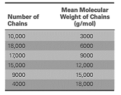
A sample of polyacrylonitrile was analyzed and the results are:

First calculate the total number of chains as:
Now, calculate the weight for each of the chain category as:
Calculate the total weight of all the chains as:
Calculate the mass fraction for each of the size range as:
Now, use formula (2) to calculate the weight average molecular weight of the polymer sample as:
The repeating unit of the polymer polyacrylonitrile is
Now, use equation (1) and calculate the degree of polymerization as:
(b)
Interpretation:
The number average molecular weight and degree of polymerization for the given polymer are to be calculated.
Concept Introduction:
The molecular weight of a polymer is not fixed. It has a certain range under which its molecular weight falls. For a linear polymer, degree of polymerization represents the average length of the polymer. Degree of polymerization is defined as:
Number average molecular weight
Here,
Answer to Problem 16.15P
The number average molecular weight for the given polymer is
The degree of polymerization for the given polymer is
Explanation of Solution
Given information:
A sample of polyacrylonitrile was analyzed and the results are:
First calculate the total number of chains as:
Calculate the fraction of chain in each of the size range as:
Now, use formula (3) to calculate the number average molecular weight of the polymer sample as:
The repeating unit of the polymer polyacrylonitrile is
Now, use equation (1) and calculate the degree of polymerization as:
Want to see more full solutions like this?
Chapter 16 Solutions
Essentials of Materials Science and Engineering, SI Edition

- (a) Determine the Nataf model for the joint PDF fxx, (xx) of the basic (physical) random variables X₁ and X, with marginal PDF's fx(x)=e, 0≤x (Exponential distribution) fx₁ (x2)=x2e-0.5x, 0≤x (Rayleigh distribution) and correlation coefficient Pxx=0.50 Note: Use Table 6 of paper by Liu and Der Kiureghian, 1986. (b) Generate a 3D surface plot and contour plot of the joint PDF fxx, (x,x) using Matlab or any other software of your choice. (c) What is the standard deviation of X2? (d) Construct a transformation from the physical X space (defined by random variables X, and X,) to the standard normal U space (defined by the statistically independent standard normal random variables (U, and U₂), i.e., U=T(X). Also describe the inverse transform X=T(U) and the Jacobian matrices J = ди θα and Ju Ox ди (e) According to the inverse transformation X = T¹ (U) and using Matlab, generate 1,000 samples from the Nataf joint PDF fxx, (x1,x2) derived in part (a). Start by generating samples of U using a…arrow_forwardBased on the results obtained, comment on the relative importance of the body and the tails of thedistributions of R and S on the probability of failure with increasing central safety factor CSF .arrow_forwardFind Vo using mesh analysisarrow_forward
- The resistance R and load effect S for a given failure mode are statistically independent random variables with marginal PDF's 1 fR (r) = 0≤r≤100 100' fs(s)=0.05e-0.05s (a) Determine the probability of failure by computing the probability content of the failure domain defined as {rarrow_forward1. The beam is supported by a roller constraint at B, which allows vertical displacement but resists axial load and moment. If the bar is subjected to the loading shown and constant El (L = 12 ft, E = 3100 ksi, I = 1728 in (rectangular section 12"x12"), w = 1 klf). Caution: pay attention to unit conversion between ft and in) x W B a. Sketch the deflected shape. L b. Determine the equations of the slope and the elastic curve using the coordinate x. First, solve this problem parametrically, and then substitute the numerical values for L, E, I, w at the end. There will be a significant penalty for solutions that do not calculate the slope and deflection as parametric functions. c. Specify the slope (in radians) at point A (parametrically and numerically). d. Specify the vertical displacement at point B (parametrically and numerically).arrow_forward4. EI is constant in the beam below (a = 12 ft, b = 5 ft, E = 29,000 ksi, I = 800 in¹ (W18x50), P = 2 kip): b Р C a. Sketch the deflected shape. b. Determine the equations of the slope and the elastic curve using the coordinates x1 and x2. c. For the AB segment, determine the maximum deflection and its location. Hint: at maximum deflection, the slope is zero. d. Specify the slope (in radians) and deflection at point C.arrow_forward3. EI is constant in the beam below (a = 10 ft, b = 5 ft, E = 29,000 ksi, I = 340 in (W14x34), Mo = 50 k. ft): Mo Mo a. Sketch the deflected shape. X2 b. Determine the equations of the slope and the elastic curve using the coordinates x1 and x2. Due to symmetry, only the left side is sufficient. Hint: symmetry requires the slope to be zero at mid span. c. Determine the maximum deflection. d. Specify the slope (in radians) at point A.arrow_forward2. EI is constant in the beam below (L = 10 ft, E = 29,000 ksi, I = 350 in (W12x45), W = 500 lb/ft): a. Sketch the deflected shape. b. Determine the equations of the slope and the elastic curve using the coordinates x1 and X2. c. Specify the slope (in radians) and deflection at point C. d. Specify the slope (in radians) at point B. -x- L 2 W C X27 L 22 Barrow_forwardPlease solve this problem as soon as possible My ID# 016948724arrow_forwardRead the paper of Khalili et al. (2004). Describe the issue raised by Jennings and Burland in using the single-value effective stress to quantify the problem of wetting-induced collapse. Use the discussion in Khalili et al. (2004) on the different ways that effective stress and yield stress change with suction to explain how wetting-induced collapse can be modeled with the single-valued effective stress. Comment on whether the soil tested by Jotisankasa (2003) would be collapsible based on the discussionarrow_forwardc) An RC circuit is given in Figure Q1.1, where Vi(t) and Vo(t) are the input and output voltages. (i) Derive the transfer function of the circuit. (ii) With a unit step change of Vi(t) applied to the circuit, derive the time response of Vo(t) with this step change. Vi(t) C₁ Vo(1) R₂ C2 C3 | R = 20 ΚΩ = 50 ΚΩ C=C2=C3=25 μF Figure Q1.1. RC circuit.arrow_forwardc) An RC circuit is given in Figure Q1. vi(t) and vo (t) are the input and output voltages. (i) Derive the transfer function of the circuit. (ii) With a unit step change vi(t) applied to the circuit, derive and sketch the time response of the circuit. R₁ R2 v₁(t) R3 C₁ v₁(t) R₁ = R₂ = 10 k R3 = 100 kn C₁ = 100 μF Figure Q1. RC circuit.arrow_forwardarrow_back_iosSEE MORE QUESTIONSarrow_forward_ios
 MATLAB: An Introduction with ApplicationsEngineeringISBN:9781119256830Author:Amos GilatPublisher:John Wiley & Sons Inc
 Essentials Of Materials Science And EngineeringEngineeringISBN:9781337385497Author:WRIGHT, Wendelin J.Publisher:Cengage,
 Industrial Motor ControlEngineeringISBN:9781133691808Author:Stephen HermanPublisher:Cengage Learning
 Basics Of Engineering EconomyEngineeringISBN:9780073376356Author:Leland Blank, Anthony TarquinPublisher:MCGRAW-HILL HIGHER EDUCATION
 Structural Steel Design (6th Edition)EngineeringISBN:9780134589657Author:Jack C. McCormac, Stephen F. CsernakPublisher:PEARSON
 Fundamentals of Materials Science and Engineering...EngineeringISBN:9781119175483Author:William D. Callister Jr., David G. RethwischPublisher:WILEY