Concept explainers
Videos
The Professional Golfers Association (PGA) maintains data on performance and earnings for members of the PGA Tour. For the 2012 season Bubba Watson led all players in total driving distance, with an average of 309.2 yards per drive. Some of the factors thought to influence driving distance are club head speed, ball speed, and launch angle. For the 2012 season Bubba Watson had an average club head speed of 124.69 miles per hour, an average ball speed of 184.98 miles per hour, and an average launch angle of 8.79 degrees. The DATAfile named PGADrivingDist contains data on total driving distance and the factors related to driving distance for 190 members of the PGA Tour (PGA Tour website, November 1, 2012). Descriptions for the variables in the data set follow.
Club Head Speed: Speed at which the club impacts the ball (mph)
Ball Speed: Peak speed of the golf ball at launch (mph)
Launch Angle: Vertical launch angle of the ball immediately after leaving the club (degrees)
Total Distance: The average number of yards per drive
- a. Develop an estimated regression equation that can be used to predict the average number of yards per drive given the club head speed.
- b. Develop an estimated regression equation that can be used to predict the average number of yards per drive given the ball speed.
- c. A recommendation has been made to develop an estimated regression equation that uses both club head speed and ball speed to predict the average number of yards per drive. Do you agree with this? Explain.
- d. Develop an estimated regression equation that can be used to predict the average number of yards per drive given the ball speed and the launch angle.
- e. Suppose a new member of the PGA Tour for 2013 has a ball speed of 170 miles per hour and a launch angle of 11 degrees. Use the estimated regression equation in part (d) to predict the average number of yards per drive for this player.
a.
Find the estimated regression equation that could be used to predict the average number of yards per drive given the club head speed.
Answer to Problem 9E
The estimated regression equation that could be used to predict the average number of yards per drive given the club head speed is
Explanation of Solution
Calculation:
The Professional Golfers Association (PGA) data consisting of information regarding to the speed at which the club impacts the ball (Club Head Speed), peak speed of the golf ball at launch (Ball Speed), Vertical Launch angle of the ball immediately after leaving the club (Launch Angle) and the average number of yards per drive (Total Distance).
Multiple linear regression model:
A multiple linear regression model is given as
Regression:
Software procedure:
Step by step procedure to get regression equation using MINITAB software is given as,
- Choose Stat > Regression > Regression > Fit Regression Model.
- Under Responses, enter the column of Total Distance.
- Under Continuous predictors, enter the columns of Club Head Speed.
- Click OK.
The output using MINITAB software is given as,
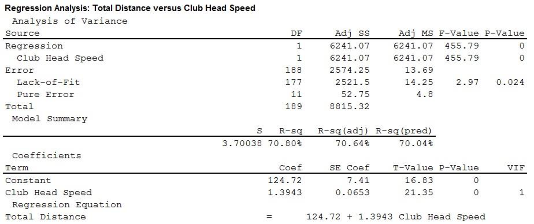
Thus, the estimated regression equation that could be used to predict the average number of yards per drive given the club head speed is
b.
Find the estimated regression equation that could be used to predict the average number of yards per drive given the ball speed.
Answer to Problem 9E
The estimated regression equation that could be used to predict the average number of yards per drive given the ball speed is
Explanation of Solution
Calculation:
Regression:
Software procedure:
Step by step procedure to get regression equation using MINITAB software is given as,
- Choose Stat > Regression > Regression > Fit Regression Model.
- Under Responses, enter the column of Total Distance.
- Under Continuous predictors, enter the columns of Ball Speed.
- Click OK.
The output using MINITAB software is given as,
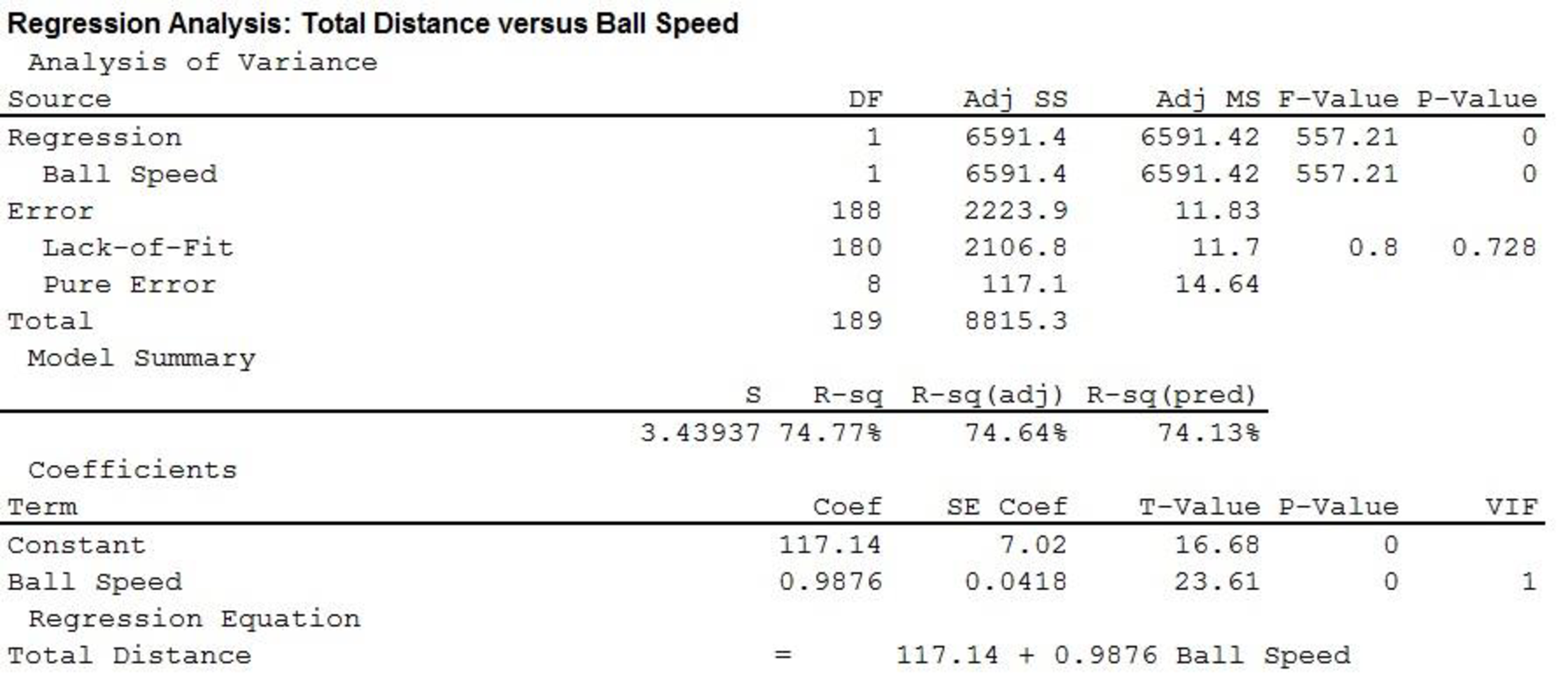
Thus, the estimated regression equation that could be used to predict the average number of yards per drive given the ball speed is
c.
Explain whether developing an estimated regression equation that uses both club head speed and ball speed to predict the average number of yards per drive, is useful.
Explanation of Solution
Calculation:
Regression:
Software procedure:
Step by step procedure to get regression equation using MINITAB software is given as,
- Choose Stat > Regression > Regression > Fit Regression Model.
- Under Responses, enter the column of Total Distance.
- Under Continuous predictors, enter the columns of Club Head Speed and Ball Speed.
- Click OK.
The output using MINITAB software is given as,
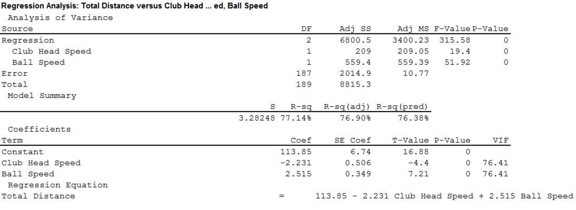
Thus, the estimated regression equation that could be used to predict the average number of yards per drive given both club head speed and ball speed is,
In the given output,
Thus, only 77.14% variability in total distance can be explained by variability in Club Head and Ball Speed.
Scatter Diagram:
Software Procedure:
Step by step procedure to obtain scatter diagram using MINITAB software is given as,
- Choose Graph > Scatter plot.
- Choose Simple, and then click OK.
- Under Y variables, enter a column of Ball Speed.
- Under X variables, enter a column of Club Head Speed.
- Click Ok.
The MINITAB output is given as,
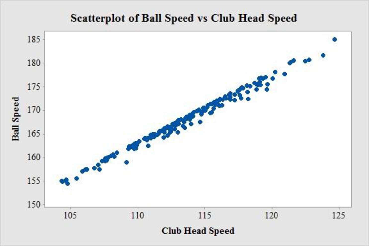
The scatter diagram exhibits a strong positive linear relationship between ball speed and club head speed. Both variables in the same model is not recommended as the linear effect of one variable describes the linear effect of the other variable. As a result, the other variable will be of little additional value. Thus, there is a chance of multicollinearity.
Thus, developing an estimated regression equation that uses both club head speed and ball speed to predict the average number of yards per drive, is not useful.
d.
Explain whether developing an estimated regression equation that uses both club head speed and launch angle to predict the average number of yards per drive.
Answer to Problem 9E
The estimated regression equation that could be used to predict the average number of yards per drive given both club head speed and Launch Angle is,
Explanation of Solution
Calculation:
Regression:
Software procedure:
Step by step procedure to get regression equation using MINITAB software is given as,
- Choose Stat > Regression > Regression > Fit Regression Model.
- Under Responses, enter the column of Total Distance.
- Under Continuous predictors, enter the columns of Club Head Speed and Launch Angle.
- Click OK.
The output using MINITAB software is given as,
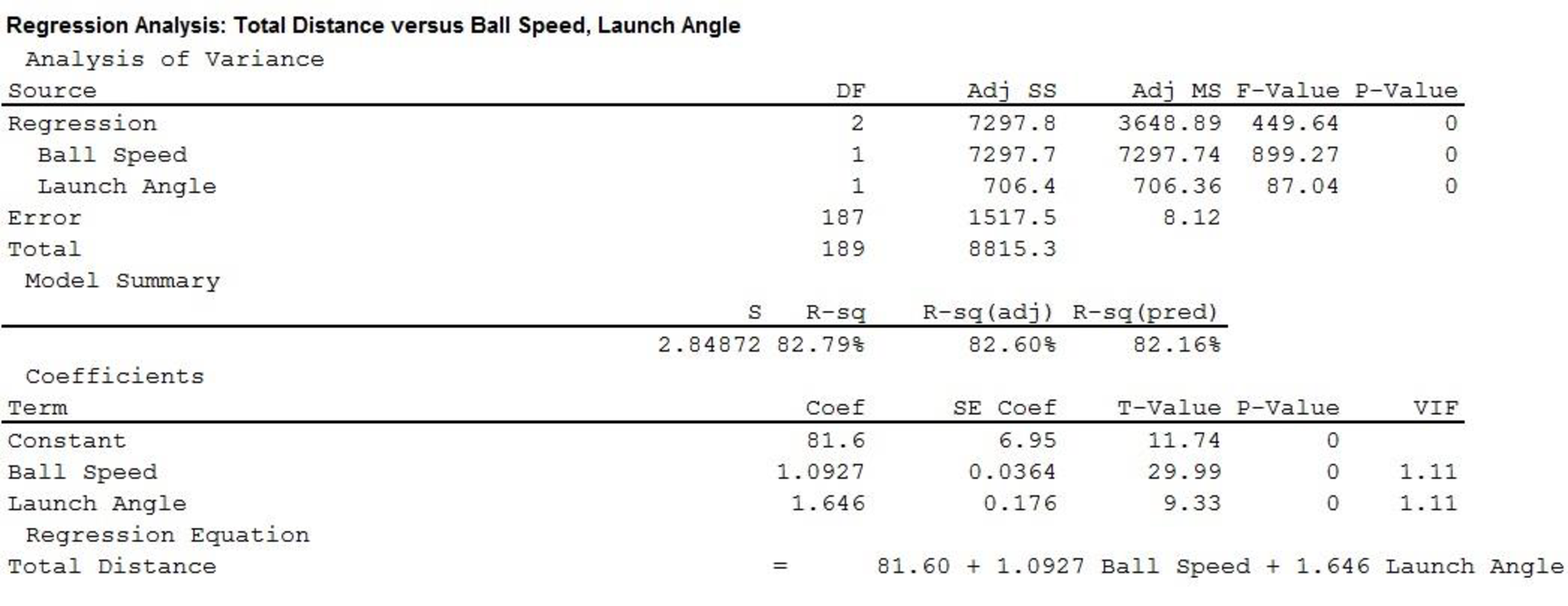
Thus, the estimated regression equation that could be used to predict the average number of yards per drive given both club head speed and Launch Angle is,
e.
Predict the average number of yards per drive for the new player using the obtained equation in part (d).
Answer to Problem 9E
The predicted average number of yards per drive for the new player is 285.465 yards.
Explanation of Solution
Calculation:
The ball speed of a new PGA player is 170 mph with launch angle of 11 degrees.
From previous part (b) it is found that estimated regression equation that could be used to predict the average number of yards per drive given both club head speed and Launch Angle is
Thus, the predicted average number of yards per drive for the new player is,
Thus, the predicted average number of yards per drive for the new player is 285.465 yards.
Want to see more full solutions like this?
Chapter 15 Solutions
Bundle: Statistics for Business & Economics, Loose-leaf Version, 13th + MindTap Business Statistics with XLSTAT, 2 terms (12 months) Printed Access Card


- Examine the Variables: Carefully review and note the names of all variables in the dataset. Examples of these variables include: Mileage (mpg) Number of Cylinders (cyl) Displacement (disp) Horsepower (hp) Research: Google to understand these variables. Statistical Analysis: Select mpg variable, and perform the following statistical tests. Once you are done with these tests using mpg variable, repeat the same with hp Mean Median First Quartile (Q1) Second Quartile (Q2) Third Quartile (Q3) Fourth Quartile (Q4) 10th Percentile 70th Percentile Skewness Kurtosis Document Your Results: In RStudio: Before running each statistical test, provide a heading in the format shown at the bottom. “# Mean of mileage – Your name’s command” In Microsoft Word: Once you've completed all tests, take a screenshot of your results in RStudio and paste it into a Microsoft Word document. Make sure that snapshots are very clear. You will need multiple snapshots. Also transfer these results to the…arrow_forward2 (VaR and ES) Suppose X1 are independent. Prove that ~ Unif[-0.5, 0.5] and X2 VaRa (X1X2) < VaRa(X1) + VaRa (X2). ~ Unif[-0.5, 0.5]arrow_forward8 (Correlation and Diversification) Assume we have two stocks, A and B, show that a particular combination of the two stocks produce a risk-free portfolio when the correlation between the return of A and B is -1.arrow_forward
- 9 (Portfolio allocation) Suppose R₁ and R2 are returns of 2 assets and with expected return and variance respectively r₁ and 72 and variance-covariance σ2, 0%½ and σ12. Find −∞ ≤ w ≤ ∞ such that the portfolio wR₁ + (1 - w) R₂ has the smallest risk.arrow_forward7 (Multivariate random variable) Suppose X, €1, €2, €3 are IID N(0, 1) and Y2 Y₁ = 0.2 0.8X + €1, Y₂ = 0.3 +0.7X+ €2, Y3 = 0.2 + 0.9X + €3. = (In models like this, X is called the common factors of Y₁, Y₂, Y3.) Y = (Y1, Y2, Y3). (a) Find E(Y) and cov(Y). (b) What can you observe from cov(Y). Writearrow_forward1 (VaR and ES) Suppose X ~ f(x) with 1+x, if 0> x > −1 f(x) = 1−x if 1 x > 0 Find VaRo.05 (X) and ES0.05 (X).arrow_forward
- Joy is making Christmas gifts. She has 6 1/12 feet of yarn and will need 4 1/4 to complete our project. How much yarn will she have left over compute this solution in two different ways arrow_forwardSolve for X. Explain each step. 2^2x • 2^-4=8arrow_forwardOne hundred people were surveyed, and one question pertained to their educational background. The results of this question and their genders are given in the following table. Female (F) Male (F′) Total College degree (D) 30 20 50 No college degree (D′) 30 20 50 Total 60 40 100 If a person is selected at random from those surveyed, find the probability of each of the following events.1. The person is female or has a college degree. Answer: equation editor Equation Editor 2. The person is male or does not have a college degree. Answer: equation editor Equation Editor 3. The person is female or does not have a college degree.arrow_forward
 Elementary Geometry For College Students, 7eGeometryISBN:9781337614085Author:Alexander, Daniel C.; Koeberlein, Geralyn M.Publisher:Cengage,
 Glencoe Algebra 1, Student Edition, 9780079039897...AlgebraISBN:9780079039897Author:CarterPublisher:McGraw Hill
 Holt Mcdougal Larson Pre-algebra: Student Edition...AlgebraISBN:9780547587776Author:HOLT MCDOUGALPublisher:HOLT MCDOUGAL