Chapter 15, Problem 64DA

a.

To determine

Check whether people can conclude that less than 40% of the districts buses are old.

Find the p-value.

Answer to Problem 64DA

Yes, people cannot conclude that less than 40% of the districts buses are old.

The p-value is 0.181.

Explanation of Solution

Calculation:

In this case, the test is to check whether less than 40% of the districts buses are old.

Let $\pi$ represents hypothesized population proportion of old buses in districts.

$\begin{array}{l}{H}_0:\pi \ge 0.40\\ H_1:\pi <0.40\end{array}$

From the data, it can be observed that the number of old buses is 28 out of 80.

The level of significance is 0.01.

Therefore, the value of z score using the table B.3: Areas under the normal curve is –2.33.

Decision rule:

Reject the null hypothesis if z < –2.326.

The sample size n is 80, p is 0.40 and the number of old buses (x) is 28.

Step-by-step procedure to find the test statistic using MINITAB software:

• Choose Stat > Basic Statistics > 1 Proportion.
• Choose Summarized data.
• In Number of events, enter 28. In Number of trials, enter 80.
• Enter Hypothesized proportion as 0.40.
• Check Options, enter Confidence level as 99.0.
• Choose greater than in alternative.
• Select Method as Normal approximation.
• Click OK in all dialogue boxes.

Output is obtained as follows:

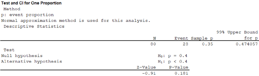
Thus, the value of the test statistic is –0.91 and the p-value is 0.181.

In this case, the critical value is –2.33 and the test statistic is –0.91.

Here, the test statistic –0.91 is greater than the critical value –2.33.

That is, –0.91 > –2.33.

Therefore, do not reject the null hypothesis.

Therefore, people cannot conclude that less than 40% of the districts buses are old.

b.

To determine

Find the median maintenance cost and the median age of the buses.

Check whether the age of the bus is related to the amount of the maintenance cost.

Answer to Problem 64DA

The median maintenance cost and the median age of the buses are $4,179 and 7.00, respectively.

Yes, the age of the bus is related to the amount of the maintenance cost.

Explanation of Solution

Calculation:

In this case, the test is to check whether the age of the bus is related to the amount of the maintenance cost.

$H_0:$ There is no relationship between age of the bus and maintenance cost.

$H_1:$ There is a relationship between age of the bus and maintenance cost.

Step-by-step procedure to find the median for age of the bus and maintenance cost using MINITAB software:

• Choose Stat > Basic Statistics > Display Descriptive Statistics.
• In Variables enter the columns Age and Maintenance cost.
• Choose option statistics, and select Median.
• Click OK.

Output using MINITAB software is obtained as follows:

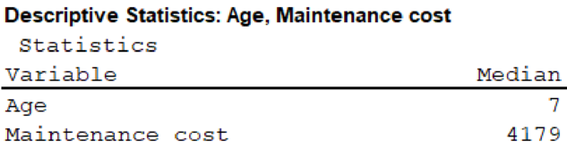
From the output, the median maintenance cost and the median age of the buses are $4,179 and 7.00, respectively.

Using the given conditions, the contingency table is obtained as follows:

High Maintenance	Age
	Lower half	Top half	Total
No	33	7	40
Yes	9	31	40
Total	42	38	80

The number of degrees of freedom is obtained as follows:

$\begin{array}{c}\text{Degrees of freedom}=\left(\text{Rows}-1\right)\left(\text{Columns}-1\right)\\ =\left(2-1\right)\left(2-1\right)\\ =1\end{array}$

Therefore, the number of degrees of freedom is 1.

Step-by-step procedure to find the critical value using MINITAB software:

• Choose Graph > Probability Distribution Plot > View Probability > OK.
• From Distribution, choose ‘Chi-Square’ distribution.
• Enter Degrees of freedom is 1.
• Click the Shaded Area tab.
• Choose Probability and Right Tail for the region of the curve to shade.
• Enter the data value as 0.01.
• Click OK.

Output using MINITAB software is obtained as follows:

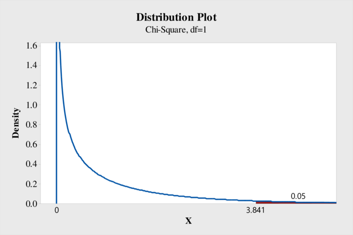
From the output, the critical value of chi-square is 3.841.

The general decision rule is reject the null hypothesis if ${\chi }^2$> critical value.

Therefore, the decision rule is reject the null hypothesis if ${\chi }^2>3.84$.

Test statistic:

Step-by-step procedure to find the test statistic using MINITAB software:

• Choose Stat > Tables > Chi-Square Test for Association.
• Choose Summarized data in a two-way table.
• In Columns containing the table, enter the columns of Lower half and Top half.
• In Rows under Labels for the table, enter the column of High Maintenance.
• Click OK.

Output is obtained as follows:

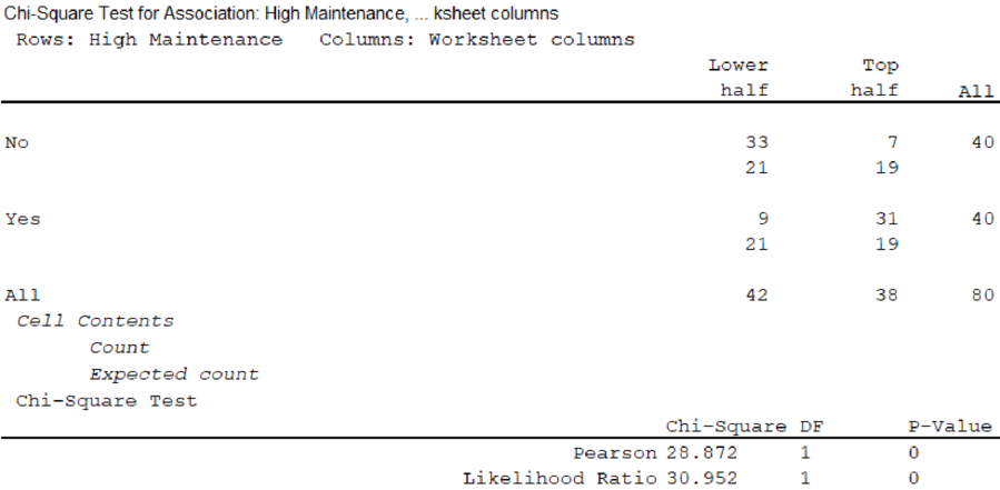
From the output, the test statistic is 28.872.

The critical value is 3.84.

Here, the test statistic is greater than the critical value.

That is, 28.872 > 3.84.

Thus, reject the null hypothesis.

Therefore, there is sufficient evidence to conclude that age of the bus is related to the amount of the maintenance cost.

c.

To determine

Check whether there is a relationship between the maintenance cost and the manufacturer of the bus.

Answer to Problem 64DA

No, there is no relationship between the maintenance cost and the manufacturer of the bus.

Explanation of Solution

Calculation:

In this case, the test is to check whether there is a relationship between the maintenance cost and the manufacturer of the bus.

$H_0:$ There is no relationship between age of the maintenance cost and manufacturer of the bus.

$H_1:$ There is a relationship between age of the maintenance cost and manufacturer of the bus.

Using the given conditions, the contingency table for the maintenance cost and manufacturer of the bus is obtained as follows:

High Maintenance	Manufacturer of the bus
	Bluebird	Keiser	Thompson	Total
No	25	13	2	40
Yes	22	12	6	40
Total	47	25	8	80

The number of degrees of freedom is obtained as follows:

$\begin{array}{c}\text{Degrees of freedom}=\left(\text{Rows}-1\right)\left(\text{Columns}-1\right)\\ =\left(2-1\right)\left(3-1\right)\\ =2\end{array}$

Therefore, the number of degrees of freedom is 2.

Step-by-step procedure to find the critical value using MINITAB software:

• Choose Graph > Probability Distribution Plot > View Probability > OK.
• From Distribution, choose ‘Chi-Square’ distribution.
• Enter Degrees of freedom is 1.
• Click the Shaded Area tab.
• Choose Probability and Right Tail for the region of the curve to shade.
• Enter the data value as 0.05.
• Click OK.

Output using MINITAB software is obtained as follows:

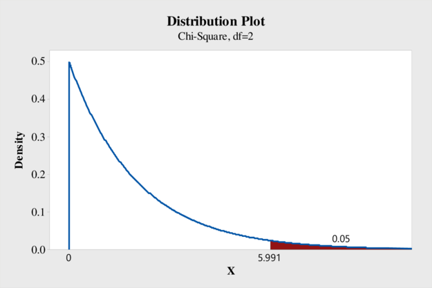
From the output, the critical value of chi-square is 5.991.

The general decision rule is reject the null hypothesis if ${\chi }^2$> critical value.

Therefore, the decision rule is reject the null hypothesis if ${\chi }^2>5.991$.

Test statistic:

Step-by-step procedure to find the test statistic using MINITAB software:

• Choose Stat > Tables > Chi-Square Test for Association.
• Choose Summarized data in a two-way table.
• In Columns containing the table, enter the columns of Lower half and Top half.
• In Rows under Labels for the table, enter the column of High Maintenance.
• Click OK.

Output is obtained as follows:

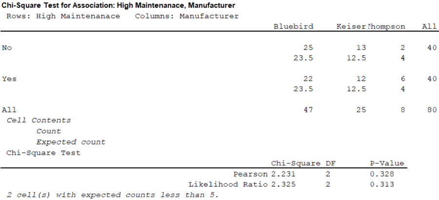
From the output, the test statistic is 2.231.

The critical value is 5.991.

Here, the test statistic is less than the critical value.

That is, 2.231 > 5.991.

Thus, do not reject the null hypothesis.

Therefore, there is no sufficient evidence to conclude that there is a relationship between the maintenance cost and the manufacturer of the bus.