Concept explainers
Videos
State the null and alternative hypothesis.
Find the degrees of freedom.
Find the critical value of chi-square from Appendix E or from Excel’s
Calculate the chi-square test statistics at 0.01 level of significance.
Interpret the p-value.
Check whether the conclusion is sensitive to the level of significance chosen, identify the cells that contribute to the chi-square test statistic and check for the small expected frequencies.
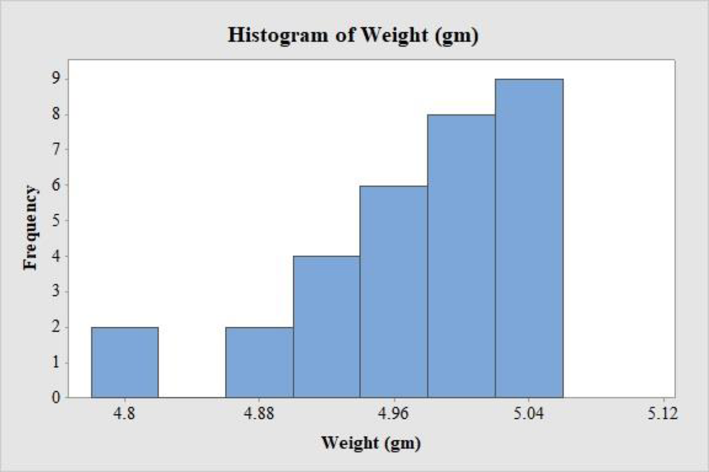
Draw histogram.
Test to obtain a probability plot with the Anderson-Darling statistic.
Interpret p-values.
Answer to Problem 40CE
The null hypothesis is:
And the alternative hypothesis is:
The degrees of freedom is 1.
The critical-value using EXCEL is 2.705543.
The chi-square test statistics at 0.1 level of significance is 0.0486.
The p-value for the hypothesis test is 0.825518.
There is enough evidence to conclude that the Circulated nickels come from a Normal population.
The conclusion is not sensitive to the level of significance chosen.
The chi-square test statistic has highest chi-square value for zero appointments.
There is no expected frequencies that are too small.
The histogram is:
The probability plot is:
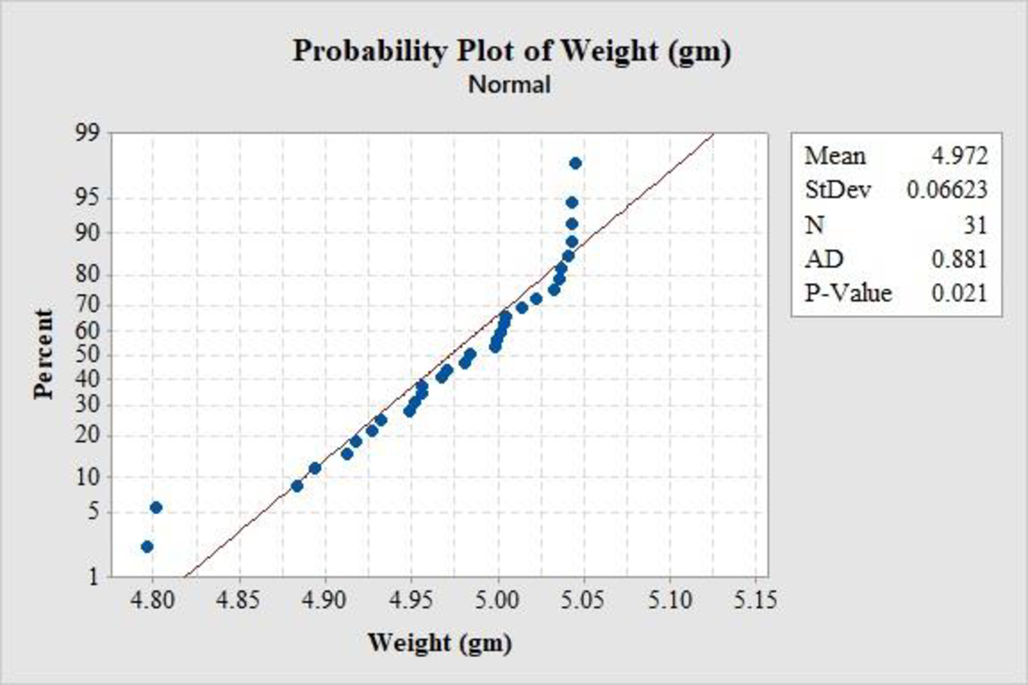
The Anderson-Darling statistics is 0.881.
The p-value is 0.021.
There is enough evidence to conclude that the Circulated nickels come from a Normal population.
Explanation of Solution
Calculation:
Results will vary.
The given information is the weights of 31 randomly chosen circulated nickels are given. There are 6 data set and pick any of them.
Here the data set F is considered
The claim is to test whether the data provide sufficient evidence to conclude that the Circulated nickels come from a Normal population. If the claim is rejected, then the Circulated nickels do not come from a Normal population.
The test hypotheses are given below:
Null hypothesis:
Alternative hypothesis:
Software procedure:
- Step by step procedure to obtain the mean and standard deviations using the MINITAB software is as follows,
- • Choose Stat > Basic Statistics>Display
Descriptive Statistics . - • Under Variables, choose 'Weight'
- • Choose Statistics, Select mean and Standard deviation.
- • Click OK.
Output obtained from MINITAB software for the data is:
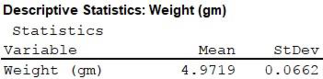
Thus, the mean and the standard deviation of the data is 4.9719 and 0.0662 respectively.
For a
Procedure for upper limit using EXCEL:
Step-by-step software procedure to obtain upper limit for first class using EXCEL is as follows:
- • Open an EXCEL file.
- • In cell A1, enter the formula “=NORM.INV(1/6,75.38,8.94)”
- Output using EXCEL software is given below:
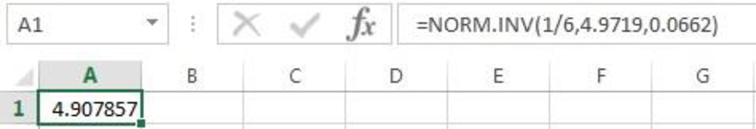
Thus, the upper limit for first class using EXCEL is 4.908.
Similarly the remaining limits can be obtained as shown below:
| Weights |
| Under 4.908 |
| 4.908–4.943 |
| 4.943–4.972 |
| 4.972–5.000 |
| 5.000–5.036 |
| 5.036 or more |
The expected frequency can be obtained by the following formula:
Where c is the number of bins and n is the sample size.
Substitute
Then the expected frequency for each bin can be obtained as shown in the table:
| Weights |
Expected Frequency |
| Under 4.908 | 5.17 |
| 4.908–4.943 | 5.17 |
| 4.943–4.972 | 5.17 |
| 4.972–5.000 | 5.17 |
| 5.000–5.036 | 5.17 |
| 5.036 or more | 5.17 |
| Total | 31 |
Frequency:
The frequencies are calculated by using the tally mark and the range of the data is from 4.796 to 5.045.
- • Based on the given information, the class intervals are under 4.908, 4.908–4.943, and so on, 5.036 or more.
- • Make a tally mark for each value in the corresponding class and continue for all values in the data.
- • The number of tally marks in each class represents the frequency, f of that class.
Similarly, the frequency of remaining classes for the emission is given below:
| Weights | Tally marks |
Observed Frequency |
| Under 4.908 | 4 | |
| 4.908–4.943 | 4 | |
| 4.943–4.972 | 6 | |
| 4.972–5.000 | 4 | |
| 5.000–5.036 | 8 | |
| 5.036 or more | 5 |
Let
The chi-square test statistics can be obtained by the formula:
Then the chi-square test statistics can be obtained as shown in the table:
| Weights |
Frequency |
Expected Frequency | ||
| Under 4.908 | 4 | 5.17 | –1.17 | 0.265 |
| 4.908–4.943 | 4 | 5.17 | –1.17 | 0.265 |
| 4.943–4.972 | 6 | 5.17 | 0.83 | 0.133 |
| 4.972–5.000 | 4 | 5.17 | –1.17 | 0.265 |
| 5.000–5.036 | 8 | 5.17 | 2.83 | 1.55 |
| 5.036 or more | 5 | 5.17 | –0.17 | 0.005 |
| Total | 31 | 31 | 0 | 2.483 |
Therefore, the chi-square test statistic is 2.483.
Degrees of freedom:
The degrees of freedom can be obtained as follows:
Where c is the number of classes and m is the number of parameters estimated. Here only 2 parameters are estimated.
Substitute 6 for c and 2 for m.
Thus, the degrees of freedom for the test is 3.
Procedure for p-value using EXCEL:
Step-by-step software procedure to obtain p-value using EXCEL software is as follows:
- • Open an EXCEL file.
- • In cell A1, enter the formula “=CHISQ.DIST.RT(2.483,3)”
- Output using EXCEL software is given below:
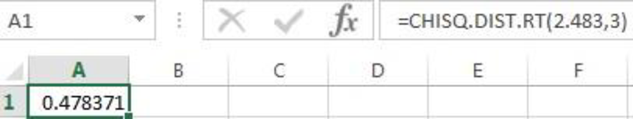
Thus, the p-value using EXCEL is 0.478.
Rejection rule:
If the p-value is less than or equal to the significance level, then reject the null hypothesis
Conclusion:
Here, the p-value is greater than the 0.01 level of significance.
That is,
Therefore, the null hypothesis is not rejected.
Thus, the data provide sufficient evidence to conclude that the Circulated nickels come from a Normal population.
Take
Here, the p-value is less than the 0.05 level of significance.
That is,
Therefore, the null hypothesis is not rejected.
Thus, the data provide sufficient evidence to conclude that the Circulated nickels come from a Normal population.
Thus, the conclusion is same for both the significance levels.
Hence, the conclusion is not sensitive to the level of significance chosen.
The class 5.000-5.036 contribute most to the chi-square test statistic.
Since all
Frequency Histogram:
Software procedure:
- Step by step procedure to draw the relative frequency histogram for mileage for 2000 using MINITAB software is as follows,
- • Choose Graph > Histogram.
- • Choose Simple.
- • Click OK.
- • In Graph variables, enter the column of 'Weight'.
- • In Scale, Choose Y-scale Type as Frequency.
- • Click OK.
- • Select Edit Scale, Enter 4.8, 4.88, 4.96, 5.04, 5.12 in Positions of ticks.
- • In Labels, Enter 4.8, 4.88, 4.96, 5.04, 5.12 41 in Specified.
- • Click OK.
Observation:
It is clear that the histogram is not symmetric. The left hand tail is little longer than the right hand tail from the maximum frequency value. Thus, there is little negative skewness on the histogram.
Software procedure:
Step by step procedure to obtain the probability plot using the MINITAB software is as follows:
- • Choose Stat > Basic Statistics > Normality Test.
- • In Variable, enter the column of 'Weights'.
- • Under Test for Normality, select the column of Anderson-Darling.
- • Click OK.
From the probability plot, it can be observed that most of the observations lies near to the straight line. Therefore, the data is from a normal distribution.
From the MINITAB output the Anderson-Darling statistics is 0.881 and the p-value is 0.021.
Conclusion:
Here, the p-value is greater than the 0.01 level of significance.
That is,
Therefore, the null hypothesis is not rejected.
Thus, the data provide sufficient evidence to conclude that the Circulated nickels come from a Normal population.
Want to see more full solutions like this?
Chapter 15 Solutions
Applied Statistics in Business and Economics


- Techniques QUAT6221 2025 PT B... TM Tabudi Maphoru Activities Assessments Class Progress lIE Library • Help v The table below shows the prices (R) and quantities (kg) of rice, meat and potatoes items bought during 2013 and 2014: 2013 2014 P1Qo PoQo Q1Po P1Q1 Price Ро Quantity Qo Price P1 Quantity Q1 Rice 7 80 6 70 480 560 490 420 Meat 30 50 35 60 1 750 1 500 1 800 2 100 Potatoes 3 100 3 100 300 300 300 300 TOTAL 40 230 44 230 2 530 2 360 2 590 2 820 Instructions: 1 Corall dawn to tha bottom of thir ceraan urina se se tha haca nariad in archerca antarand cubmit Q Search ENG US 口X 2025/05arrow_forwardThe table below indicates the number of years of experience of a sample of employees who work on a particular production line and the corresponding number of units of a good that each employee produced last month. Years of Experience (x) Number of Goods (y) 11 63 5 57 1 48 4 54 45 3 51 Q.1.1 By completing the table below and then applying the relevant formulae, determine the line of best fit for this bivariate data set. Do NOT change the units for the variables. X y X2 xy Ex= Ey= EX2 EXY= Q.1.2 Estimate the number of units of the good that would have been produced last month by an employee with 8 years of experience. Q.1.3 Using your calculator, determine the coefficient of correlation for the data set. Interpret your answer. Q.1.4 Compute the coefficient of determination for the data set. Interpret your answer.arrow_forwardQ.3.2 A sample of consumers was asked to name their favourite fruit. The results regarding the popularity of the different fruits are given in the following table. Type of Fruit Number of Consumers Banana 25 Apple 20 Orange 5 TOTAL 50 Draw a bar chart to graphically illustrate the results given in the table.arrow_forward
- Q.2.3 The probability that a randomly selected employee of Company Z is female is 0.75. The probability that an employee of the same company works in the Production department, given that the employee is female, is 0.25. What is the probability that a randomly selected employee of the company will be female and will work in the Production department? Q.2.4 There are twelve (12) teams participating in a pub quiz. What is the probability of correctly predicting the top three teams at the end of the competition, in the correct order? Give your final answer as a fraction in its simplest form.arrow_forwardQ.2.1 A bag contains 13 red and 9 green marbles. You are asked to select two (2) marbles from the bag. The first marble selected will not be placed back into the bag. Q.2.1.1 Construct a probability tree to indicate the various possible outcomes and their probabilities (as fractions). Q.2.1.2 What is the probability that the two selected marbles will be the same colour? Q.2.2 The following contingency table gives the results of a sample survey of South African male and female respondents with regard to their preferred brand of sports watch: PREFERRED BRAND OF SPORTS WATCH Samsung Apple Garmin TOTAL No. of Females 30 100 40 170 No. of Males 75 125 80 280 TOTAL 105 225 120 450 Q.2.2.1 What is the probability of randomly selecting a respondent from the sample who prefers Garmin? Q.2.2.2 What is the probability of randomly selecting a respondent from the sample who is not female? Q.2.2.3 What is the probability of randomly…arrow_forwardTest the claim that a student's pulse rate is different when taking a quiz than attending a regular class. The mean pulse rate difference is 2.7 with 10 students. Use a significance level of 0.005. Pulse rate difference(Quiz - Lecture) 2 -1 5 -8 1 20 15 -4 9 -12arrow_forward
- The following ordered data list shows the data speeds for cell phones used by a telephone company at an airport: A. Calculate the Measures of Central Tendency from the ungrouped data list. B. Group the data in an appropriate frequency table. C. Calculate the Measures of Central Tendency using the table in point B. D. Are there differences in the measurements obtained in A and C? Why (give at least one justified reason)? I leave the answers to A and B to resolve the remaining two. 0.8 1.4 1.8 1.9 3.2 3.6 4.5 4.5 4.6 6.2 6.5 7.7 7.9 9.9 10.2 10.3 10.9 11.1 11.1 11.6 11.8 12.0 13.1 13.5 13.7 14.1 14.2 14.7 15.0 15.1 15.5 15.8 16.0 17.5 18.2 20.2 21.1 21.5 22.2 22.4 23.1 24.5 25.7 28.5 34.6 38.5 43.0 55.6 71.3 77.8 A. Measures of Central Tendency We are to calculate: Mean, Median, Mode The data (already ordered) is: 0.8, 1.4, 1.8, 1.9, 3.2, 3.6, 4.5, 4.5, 4.6, 6.2, 6.5, 7.7, 7.9, 9.9, 10.2, 10.3, 10.9, 11.1, 11.1, 11.6, 11.8, 12.0, 13.1, 13.5, 13.7, 14.1, 14.2, 14.7, 15.0, 15.1, 15.5,…arrow_forwardPEER REPLY 1: Choose a classmate's Main Post. 1. Indicate a range of values for the independent variable (x) that is reasonable based on the data provided. 2. Explain what the predicted range of dependent values should be based on the range of independent values.arrow_forwardIn a company with 80 employees, 60 earn $10.00 per hour and 20 earn $13.00 per hour. Is this average hourly wage considered representative?arrow_forward
- The following is a list of questions answered correctly on an exam. Calculate the Measures of Central Tendency from the ungrouped data list. NUMBER OF QUESTIONS ANSWERED CORRECTLY ON AN APTITUDE EXAM 112 72 69 97 107 73 92 76 86 73 126 128 118 127 124 82 104 132 134 83 92 108 96 100 92 115 76 91 102 81 95 141 81 80 106 84 119 113 98 75 68 98 115 106 95 100 85 94 106 119arrow_forwardThe following ordered data list shows the data speeds for cell phones used by a telephone company at an airport: A. Calculate the Measures of Central Tendency using the table in point B. B. Are there differences in the measurements obtained in A and C? Why (give at least one justified reason)? 0.8 1.4 1.8 1.9 3.2 3.6 4.5 4.5 4.6 6.2 6.5 7.7 7.9 9.9 10.2 10.3 10.9 11.1 11.1 11.6 11.8 12.0 13.1 13.5 13.7 14.1 14.2 14.7 15.0 15.1 15.5 15.8 16.0 17.5 18.2 20.2 21.1 21.5 22.2 22.4 23.1 24.5 25.7 28.5 34.6 38.5 43.0 55.6 71.3 77.8arrow_forwardIn a company with 80 employees, 60 earn $10.00 per hour and 20 earn $13.00 per hour. a) Determine the average hourly wage. b) In part a), is the same answer obtained if the 60 employees have an average wage of $10.00 per hour? Prove your answer.arrow_forward
 MATLAB: An Introduction with ApplicationsStatisticsISBN:9781119256830Author:Amos GilatPublisher:John Wiley & Sons Inc
 Probability and Statistics for Engineering and th...StatisticsISBN:9781305251809Author:Jay L. DevorePublisher:Cengage Learning
 Statistics for The Behavioral Sciences (MindTap C...StatisticsISBN:9781305504912Author:Frederick J Gravetter, Larry B. WallnauPublisher:Cengage Learning
 Elementary Statistics: Picturing the World (7th E...StatisticsISBN:9780134683416Author:Ron Larson, Betsy FarberPublisher:PEARSON
 The Basic Practice of StatisticsStatisticsISBN:9781319042578Author:David S. Moore, William I. Notz, Michael A. FlignerPublisher:W. H. Freeman
 Introduction to the Practice of StatisticsStatisticsISBN:9781319013387Author:David S. Moore, George P. McCabe, Bruce A. CraigPublisher:W. H. Freeman