
Concept explainers
Videos
Matt Kenseth won the 2012 Daytona 500, the most important race of the NASCAR season. His win was no surprise because for the 2011 season he finished fourth in the point standings with 2330 points, behind Tony Stewart (2403 points), Carl Edwards (2403 points), and Kevin Harvick (2345 points). In 2011 he earned $6,183,580 by winning three Poles (fastest driver in qualifying), winning three races, finishing in the top five 12 times, and finishing in the top ten 20 times. NASCAR’s point system in 2011 allocated 43 points to the driver who finished first, 42 points to the driver who finished second, and so on down to 1 point for the driver who finished in the 43rd position. In addition any driver who led a lap received 1 bonus point, the driver who led the most laps received an additional bonus point, and the race winner was awarded 3 bonus points. But, the maximum number of points a driver could earn in any race was 48. Table 15.13 shows data for the 2011 season for the top 35 drivers (NASCAR website).
Managerial Report
- 1. Suppose you wanted to predict Winnings ($) using only the number of poles won (Poles), the number of wins (Wins), the number of top five finishes (Top 5), or the number of top ten finishes (Top 10). Which of these four variables provides the best single predictor of winnings?
- 2. Develop an estimated regression equation that can be used to predict Winnings ($) given the number of poles won (Poles), the number of wins (Wins), the number of top five finishes (Top 5), and the number of top ten (Top 10) finishes. Test for individual significance and discuss your findings and conclusions.
- 3. Create two new independent variables: Top 2–5 and Top 6–10. Top 2–5 represents the number of times the driver finished between second and fifth place and Top 6–10 represents the number of times the driver finished between sixth and tenth place. Develop an estimated regression equation that can be used to predict Winnings ($) using Poles, Wins, Top 2–5, and Top 6–10. Test for individual significance and discuss your findings and conclusions.
TABLE 15.13 Nascar Results for the 2011 Season
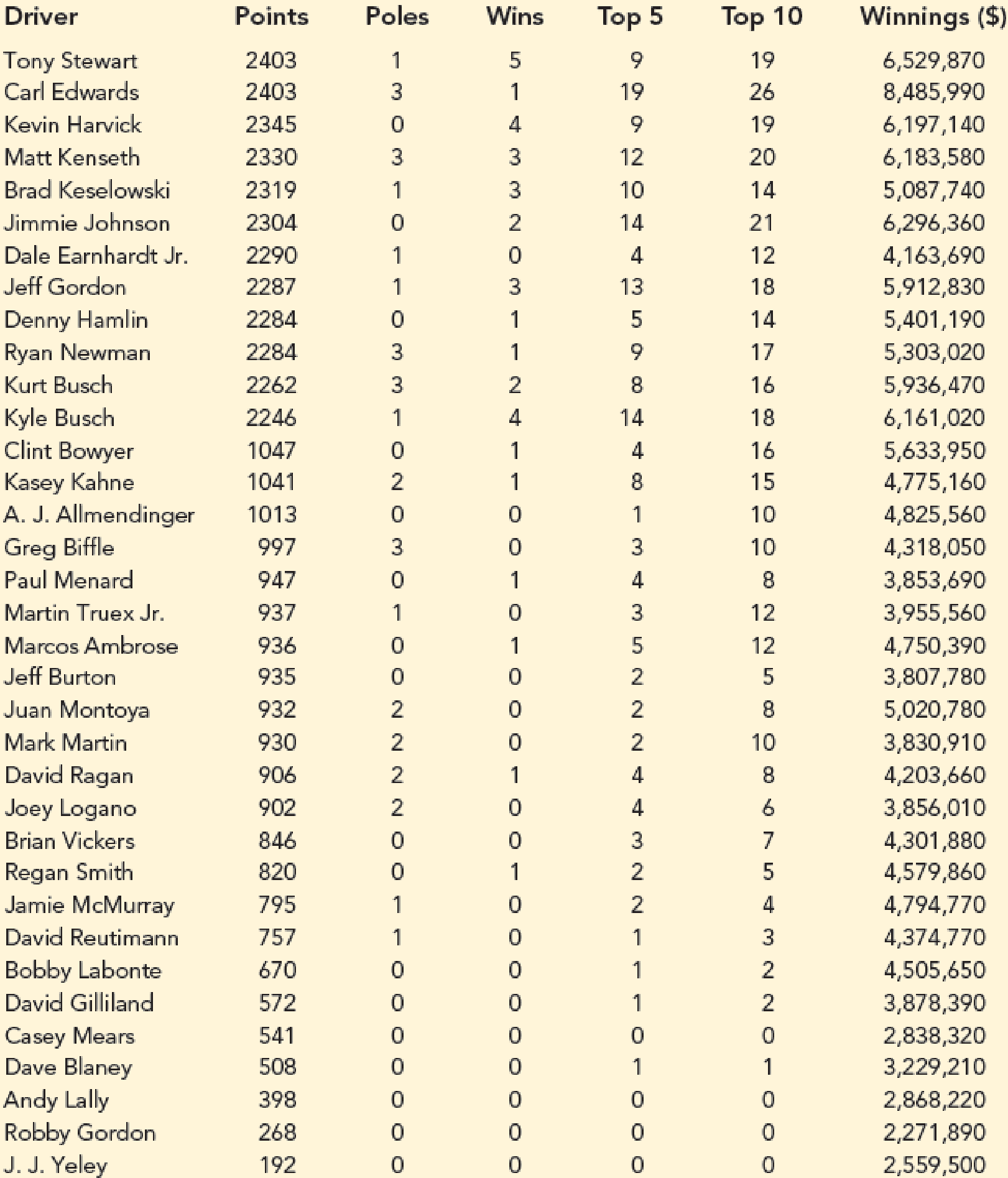
Source: NASCAR website, February 28, 2011. (https://www.nascar.com/)
- 4. Based upon the results of your analysis, what estimated regression equation would you recommend using to predict Winnings ($)? Provide an interpretation of the estimated regression coefficients for this equation.

Trending nowThis is a popular solution!

Chapter 15 Solutions
Essentials Of Statistics For Business & Economics


- 38. Possible values of X, the number of components in a system submitted for repair that must be replaced, are 1, 2, 3, and 4 with corresponding probabilities .15, .35, .35, and .15, respectively. a. Calculate E(X) and then E(5 - X).b. Would the repair facility be better off charging a flat fee of $75 or else the amount $[150/(5 - X)]? [Note: It is not generally true that E(c/Y) = c/E(Y).]arrow_forward74. The proportions of blood phenotypes in the U.S. popula- tion are as follows:A B AB O .40 .11 .04 .45 Assuming that the phenotypes of two randomly selected individuals are independent of one another, what is the probability that both phenotypes are O? What is the probability that the phenotypes of two randomly selected individuals match?arrow_forward53. A certain shop repairs both audio and video compo- nents. Let A denote the event that the next component brought in for repair is an audio component, and let B be the event that the next component is a compact disc player (so the event B is contained in A). Suppose that P(A) = .6 and P(B) = .05. What is P(BA)?arrow_forward
- 26. A certain system can experience three different types of defects. Let A;(i = 1,2,3) denote the event that the sys- tem has a defect of type i. Suppose thatP(A1) = .12 P(A) = .07 P(A) = .05P(A, U A2) = .13P(A, U A3) = .14P(A2 U A3) = .10P(A, A2 A3) = .011Rshelfa. What is the probability that the system does not havea type 1 defect?b. What is the probability that the system has both type 1 and type 2 defects?c. What is the probability that the system has both type 1 and type 2 defects but not a type 3 defect? d. What is the probability that the system has at most two of these defects?arrow_forwardThe following are suggested designs for group sequential studies. Using PROCSEQDESIGN, provide the following for the design O’Brien Fleming and Pocock.• The critical boundary values for each analysis of the data• The expected sample sizes at each interim analysisAssume the standardized Z score method for calculating boundaries.Investigators are evaluating the success rate of a novel drug for treating a certain type ofbacterial wound infection. Since no existing treatment exists, they have planned a one-armstudy. They wish to test whether the success rate of the drug is better than 50%, whichthey have defined as the null success rate. Preliminary testing has estimated the successrate of the drug at 55%. The investigators are eager to get the drug into production andwould like to plan for 9 interim analyses (10 analyzes in total) of the data. Assume thesignificance level is 5% and power is 90%.Besides, draw a combined boundary plot (OBF, POC, and HP)arrow_forwardPlease provide the solution for the attached image in detailed.arrow_forward
- 20 km, because GISS Worksheet 10 Jesse runs a small business selling and delivering mealie meal to the spaza shops. He charges a fixed rate of R80, 00 for delivery and then R15, 50 for each packet of mealle meal he delivers. The table below helps him to calculate what to charge his customers. 10 20 30 40 50 Packets of mealie meal (m) Total costs in Rands 80 235 390 545 700 855 (c) 10.1. Define the following terms: 10.1.1. Independent Variables 10.1.2. Dependent Variables 10.2. 10.3. 10.4. 10.5. Determine the independent and dependent variables. Are the variables in this scenario discrete or continuous values? Explain What shape do you expect the graph to be? Why? Draw a graph on the graph provided to represent the information in the table above. TOTAL COST OF PACKETS OF MEALIE MEAL 900 800 700 600 COST (R) 500 400 300 200 100 0 10 20 30 40 60 NUMBER OF PACKETS OF MEALIE MEALarrow_forwardLet X be a random variable with support SX = {−3, 0.5, 3, −2.5, 3.5}. Part ofits probability mass function (PMF) is given bypX(−3) = 0.15, pX(−2.5) = 0.3, pX(3) = 0.2, pX(3.5) = 0.15.(a) Find pX(0.5).(b) Find the cumulative distribution function (CDF), FX(x), of X.1(c) Sketch the graph of FX(x).arrow_forwardA well-known company predominantly makes flat pack furniture for students. Variability with the automated machinery means the wood components are cut with a standard deviation in length of 0.45 mm. After they are cut the components are measured. If their length is more than 1.2 mm from the required length, the components are rejected. a) Calculate the percentage of components that get rejected. b) In a manufacturing run of 1000 units, how many are expected to be rejected? c) The company wishes to install more accurate equipment in order to reduce the rejection rate by one-half, using the same ±1.2mm rejection criterion. Calculate the maximum acceptable standard deviation of the new process.arrow_forward
- 5. Let X and Y be independent random variables and let the superscripts denote symmetrization (recall Sect. 3.6). Show that (X + Y) X+ys.arrow_forward8. Suppose that the moments of the random variable X are constant, that is, suppose that EX" =c for all n ≥ 1, for some constant c. Find the distribution of X.arrow_forward9. The concentration function of a random variable X is defined as Qx(h) = sup P(x ≤ X ≤x+h), h>0. Show that, if X and Y are independent random variables, then Qx+y (h) min{Qx(h). Qr (h)).arrow_forward
 Algebra: Structure And Method, Book 1AlgebraISBN:9780395977224Author:Richard G. Brown, Mary P. Dolciani, Robert H. Sorgenfrey, William L. ColePublisher:McDougal Littell
 Algebra for College StudentsAlgebraISBN:9781285195780Author:Jerome E. Kaufmann, Karen L. SchwittersPublisher:Cengage Learning
 Intermediate AlgebraAlgebraISBN:9781285195728Author:Jerome E. Kaufmann, Karen L. SchwittersPublisher:Cengage Learning